


Document Actions
gvSIG-Desktop 1.10. Nuevas funcionalidades
- NavTable
- Leyenda de gráficos
- Introducción
- Leyenda de tartas
- Introducción
- Visualización y selección del diagrama de tartas
- Opciones del tamaño de los diagramas
- Dibujar diagramas de tartas sólo en las geometrías seleccionadas
- Leyenda de barras
- Sextante
- Introducción
- La caja de herramientas de Sextante
- Introduction
- Diálogo de algoritmos
- Objetos de datos generados por los algoritmos de Sextante
- Ayuda contextual
- Modelador gráfico
- Introducción
- Definición de entradas
- Definición de procesos
- Edición del modelo sobre el lienzo
- Almacenamiento y recuperación de modelos
- Interfaz de procesos batch
- Introducción
- La tabla de parámetros
- Rellenando la tabla de parámetros
- Estableciendo las características de las salidas raster
- Ejecutando el proceso por lotes
- Procesos por lotes con capas ya cargadas
- Interface de línea de comandos
- Introducción
- La interfaz
- Obtener información sobre los algoritmos de análisis geográfico
- Ejecutando algoritmos
- Ajustar las características de la capa raster de salida
- El historial de procesos
NavTable
Introducción
¿ Qué es NavTable ?
NavTable is a gvSIG extension to display in an agile way the alphanumeric elements of vectorial layers. It allows seeing the features of an element in a vertical table besides editing, navigating and quick filtering the values of a layer.

NavTable is released under a GPL v3 license. It has been created by CartoLab, the Cartographic Laboratory from University of A Coruña. Feel free to send us comments, suggestions, bug reports, etc.
Listado de características
- Display data from vectorial layers in vertical align
- Edit alphanumeric values (tested with ESRI Shapefile and PostGIS)
- Navigate between elements: next, previous, ...
- Allow to navigate only by selected elements
- Zoom to the elements: manual and automatic
- Allow zoom with fixed scale
- Select and unselect elements
- Alphanumeric editing of values
- Copy attributes from last register or from selected
- Create and drop elements
- Length and area of a element is calculated
- Available in spanish, galician, english and french.
Aspectos técnicos
NavTable was designed following a modular architecture, which allow to extend their functionalities in an easy way plus using it to display personalized forms.
Its center panel is easily adaptable by injecting other forms to display, edit and even process the data. See next figure to learn the possibilities of this approach:

Bear in mind that the code of NavTable is publicly available in the project website so that you can download and adapt it.
Instrucciones de uso
Introducción
To activate NavTable you must select a vector layer in the gvSIG ToC (Table of Contents) and click the button NavTable  .
.
NavTable interface has the following areas:
- Top: basic adjustments and filter checkboxes.
- Central: view and edit data in each record.
- Bottom: navigate bar, save button and others practical buttons.

NavTable can be used for editing and display alpha-numeric tables, which have no associated geometry. For these cases, NavTable icon in the toolbar will be blue  . The title of the NavTable window for tables without geometry has a '*' to distinguish it from normal tables.
Navegación
NavTable scrolls through the records and features in a friendly way. You will find the navigation bar at the bottom of NavTable's window.

With these buttons you can:
- Go to the first record
- Go to the previous record
- Go to the next record
- Go to the last record
- Go to any record using the box located between the buttons described above. It shows the number of the records you're currently viewing. If you enter a new value here you will see the corresponding record. Next to the position of the box there is a number indicating the total amount of records in the table.
If you are working in the central area of NavTable (click on any row) you can use the buttons “right”or “left”, “home” or “end” to change the record that you want to see.
Selecting elements
If you click on the checkbox "selected" the navigation buttons will work only for features that are previous selected. If a feature is selected, the bottom area of the NavTable Window will be highlighted in yellow. In between parentheses the number of selected records can be seen next to the whole number of records.

In this image you see an example explaining how this function works: record 8 for a layer with 20 records is displayed where 7 records are selected.
If the checkbox "selected" is activated without any selected feature, all records will be shown empty and the box will not display any number. and
 .
.
The option "select" is another interesting tool you can find next to "selected" in the Nav Table menu. If you activate the checkbox next to "select", the attributes you are visualizing will be selected and highlighted in the view. In the case that other features were selected, this option will turn them unselected and will select only the register you are visualizing.
On top of the NavTable Window there is the button "Filter" . If you press it, a dialogue window will appear in which you can define exactly what you want to select (attributes and calculations). If you click on "clear selection"
 all selections will be turned off and no features will be selected.
Zoom to feature
If you click on the zoom button  the feature will be displayed in the center of the view, referring to the record you are working with at that time. The scale of the view will be changed to have a good visualization of the data. In case you are working with a point layer, a scale size will be chosen that allows to see also the surroundings of the point.

With help of the button "always zoom" next to the checkbox "select", Navtable will zoom to each feature referring to the record you are visualizing. If you click on "fixed scale" as well, Navtable will zoom to the feature and display it in the center of the view, but the scale will always remain the same. It is possible to change the scale value introducing a new one in the "scale bar" of gvSIG. This is shown on the buttom right of the gvSIG view, next to where the coordinates are displayed.
Tip: The options "always zoom" or "fixed scale" together with "select" is a very interesting way of navigate through the features of a layer.
Edición
The main new functionality in Navtable is that you don't need to start the editing mode for a layer if you want to edit it. You should follow these steps to edit the table:
- Make double click on the register you wish to work with (or click on the space bar). Now you are in editing modus and you will be able to modify this record.
- Modify the data by entering a new value
- Click on the "save" button
 .
.
After that, the new value will be saved. It's important to consider these special cases if you want to save the edition:
- with boolean fields you can only use true or false (the expression is not case sensitive). If you enter another value, the original one will be saved.
- If you try to save a value into a not appropriate field (for example from type „text“ into type „numerical“), the original value will be written.
- If you want to save an empty text, the default value will be saved. But if the field is from type „string“, the record will be saved with an empty value.
With Navtable it is also possible to use options for advanced editing. For example you can copy and paste records. For that you should select the record you want to copy first and click then on the button "copy selected feature"  . The data will be modified when you click on the button "save".
Removing records
It is possible to delete the record you are visualizing with Navtable if you click on the button "delete feature"  . If this record has an associated geometry feature (graphical element), this one will be also deleted.
Adding records to alphanumerical tables
For tables which aren't associated to a layer, Navtable has this button  . If you click on it, after the last one of the table a new record will appear.
Visualización de nombres largos
As you know, the dbf format doesn't allow field names with more than 10 characters. This limitation could be solved using alias for these fields. This option is also available for layers stored in a geodatabase.
If you wish to use this functionality you will need to create a text file with the same name as the layer in which you want to use "alias" names. Save this text file in the folder "alias" that was created when installing Navtable.
When installing gvSIG, a folder with the name gvSIG will also be created:
On Windows it is usually installed here "C:Documents and Settingsuser"

On GNU/Linux you will find it here: "/home/user/gvSIG"
When installing Navtable, a folder with the Name "Navtable" is saved to the "gvSIG" folders. At the Navtable folder you will find the "Alias" one, where you should save the text file mentioned above.

In this file you can define long names or alias for the field names.
Name_original_field=long_name
It's only necessary to describe a row for the fields you want to define an alias name for. The order of the lines isn't important, that means, you don't need to follow the same sequence like the field's names of the table.
When Navtable is opened, the according "alias" text file will be found automatically. If new names for the fields are available there, Navtable will use these ones instead of the original names.
Example: There is a dbf file with the following fields:

We define an alias text file with the same name as the shape file: Afg_district.alias in this case. In this file we will write the following text:
prov_code=province code
distr_code=district code
This file Afg_district.alias will be saved in the same folder as the file Afg_district.shp. Now we can open the table of this layer with Navtable and can see the following:

Important for Windows:
Windows doesn't show the file extension by default. For this reason for a new alias text file the name of the file will be probably name_layer.alias.txt and Navtable will not be able to read this alias file.
In order to have a correct result for this functionality we recommend you to deactivate the option hide hidden files and folders. You can make this in Windows Explorer: Extras > File Options > View > Advanced Settings > Hidden Files and Folders
Más información sobre NavTable
NavTable is hosted by the OSOR Forge [1]. On this page you can find useful information about the project and also related documents, mailing lists, bug reporting system, etc.
In the section "Future Work" on the project website you will find some of the things we want to incorporate in NavTable in the near future.
| [1] | http://navtable.forge.osor.eu/ |
Leyenda de gráficos
Introducción
Chart or diagram legends are intended to provide a visual representation of data in a table, thereby communicating a lot of information very easily.
In particular this extension allows two types of legends to be constructed:
- The first one is represented by circular diagrams known as Pie Charts. The pie chart shows the proportional size of the elements of a data series, based on the sum of its parts, and with each sector representing the value of a particular field. It always shows only one data series and is useful when you want to emphasize a significant element.
- The second type of legend is represented by diagrams known as Bar Charts or Bar Graphs. A bar graph, also known as a column graph, is a diagram containing rectangular bars with lengths proportional to the values they represent. Bar graphs are used to compare two or more values.
Leyenda de tartas
Introducción
The new pie chart legend extends the functionality of existing gvSIG legends, and can be found along with the rest of the legends in the Multiple Attributes section.
Visualización y selección del diagrama de tartas
The pie legend is located in the Multiple attributes section of the legend tree, and can be used to represent several attributes at once. To access it, right-click on the layer name to open the Properties and then select the symbols tab.
The following options are available for configuring the pie charts:
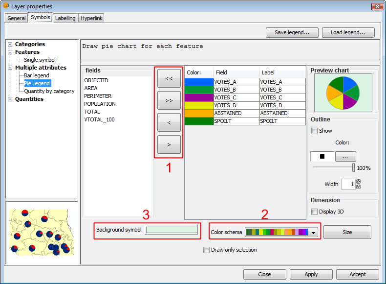
Symbols. Pie legend
Fields: You can choose which of the layer's fields to represent, provided they are numeric. With these fields you can:
- Add all fields.
- Delete all fields.
- Add the selected fields.
- Delete the selected fields.
To do this click on the buttons shown in the image above (Box 1).
Colour scheme: You can change the default colour scheme for the pies. To do this select the desired "Colour scheme" from the drop-down list, as shown in the image above (Box 2).
Change the colour: In addition it is possible to change the colour of pie slices once they have been added.
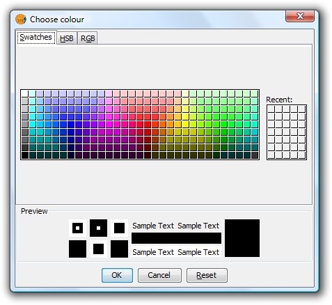
Once the default colour scheme has been chosen, the colour of a pie slice can be changed by double-clicking on its color.
The following dialog is displayed where you can select a colour sample or set it yourself (HSB, RGB).

Symbols. Color Selection
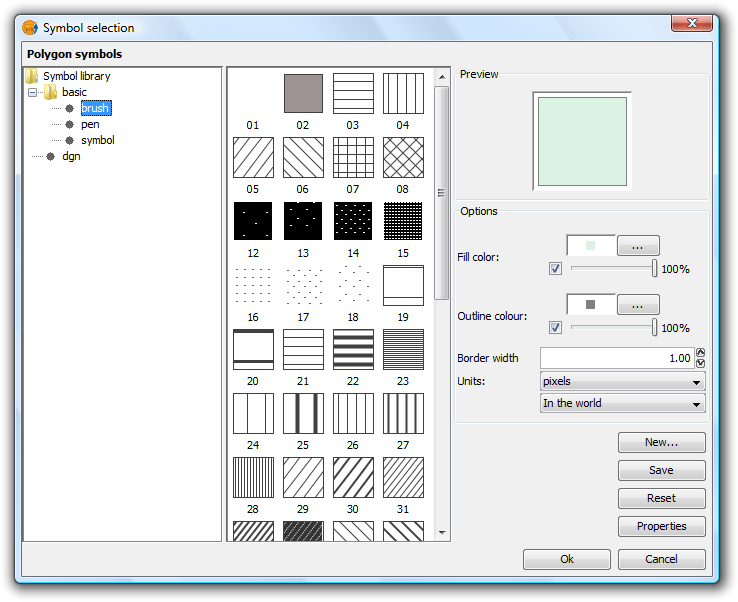
Background symbol: You can change the symbol of the background geometries by clicking on the symbol to open the symbol editor (pictured above, Box 3).

Symbols. Symbol Selector
Outline: You can display an outline with a specified colour and thickness around the pie slices. Tick the "Show" check box to draw outlines around the pie sectors.
Dimension: Tick the check box to display the pie in 3D. By default the pie is drawn in 2D.
Preview chart: Any changes made are reflected on the chart preview.
Opciones del tamaño de los diagramas
Click the 'Size' button located in the pie legend configuration screen.

Pie Legend. Size button
Clicking this will open the following dialog:
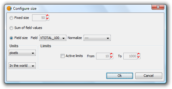
Pie Legend. Configuring size
There are three options for setting the size of the diagrams:
- Fixed Size: All the pie charts will have the size indicated here.
- Sum of field values: The size of the pie charts is obtained from the sum of all the records of the fields making up the chart.
- Field size: The size is obtained from the selected field and can be normalized if so desired.
In addition to setting the size of the pie, the units can also be specified.
Units: Select units (meters, pixels ...) and representation (in the world or print layout), depending on your requirements. If the units are set to "in the world" then the size will depend on the View's zoom level, while selecting "print layout" results in a fixed size, both on the screen and when printed.
Active Limits: Limits can be specified if the size of the chosen field size is not set to the "Fixed Size" option.
Activating limits for the other options sets the minimum and maximum values of a particular measure (Sum of field values or Field size). Taking the limits into account, the intermediate field values are calculated in proportion to the values of the records of the field, or to the sum of the field values.
Dibujar diagramas de tartas sólo en las geometrías seleccionadas
This option is used to restrict the drawing of pie charts to selected geometries.
The geometries can be selected either before or after configuring the pie chart size and display options.
In order to represent pie charts for selected geometries, simply activate the check box Draw only selection in the pie legend configuration dialog.

Check to display pie charts for selected geometries only
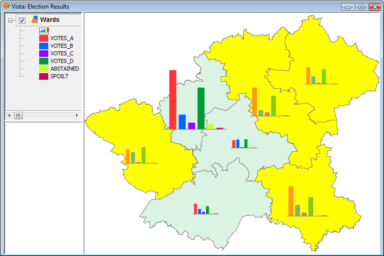
The following image shows an example in which pie charts are only shown for selected geometries (shown in yellow).
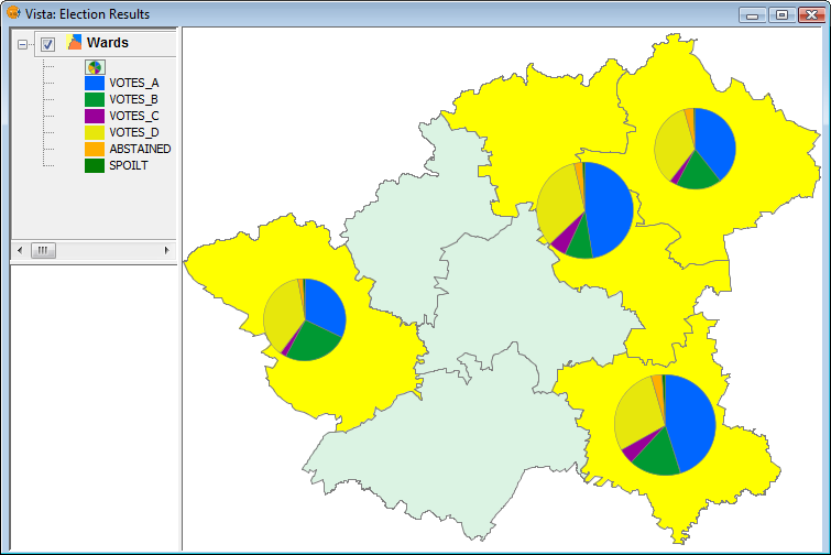
Example showing pie charts for selected geometries
Leyenda de barras
Introducción
The bar chart legend extends the functionality of existing gvSIG legends and can be found, like the pie chart, in the Multiple Attributes section.
Visualización y selección del diagrama de barras
The bar legend is located the Multiple Attributes section of the legend tree, and can be used to represent several attributes at once. To access it, right-click on the layer name to open the Properties, then select the Symbols tab.
The following options are available for configuring bar charts:
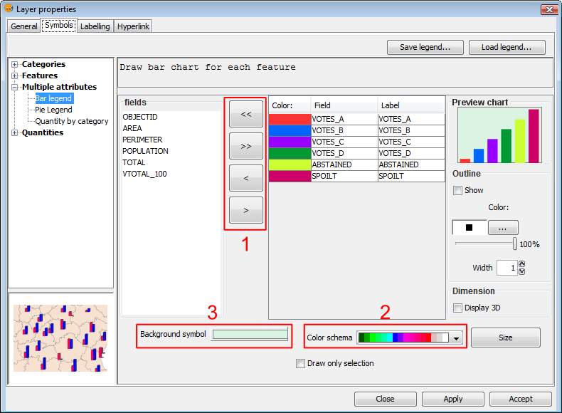
Symbols. Legend bar
Fields: You can choose which of the layer's fields to represent, provided they are numeric. With these fields you can:
- Add all fields.
- Delete all fields.
- Add the selected fields.
- Delete the selected fields.
To do this click on the buttons shown in the image above (Box 1).
Colour scheme: You can change the default colour scheme for the bars. To do this, select the desired "Colour scheme" from the drop-down list, as shown in the image above (Box 2).
Change the colour: In addition it is possible to change the colour of bars once they have been added.
Once the default colour scheme has been chosen, the colour of a bar can be changed by double-clicking on its color tile.
You can use the following dialog to select a colour sample, or set it yourself (HSB, RGB).
Symbols. Color Selection
Background symbol: You can change the symbol of the background geometries by clicking on the symbol to open the symbol editor (pictured above, Box 3).
Symbols. Symbol Selector
Outline: You can display an outline with a specified colour and thickness around the bars. Tick the "Show" check box to draw outlines around the bars.
Dimension: Tick the check box to display the bars in 3D. By default the bars are drawn in 2D.
Preview chart: Any changes made are reflected on the chart preview.
Opciones del tamaño de los diagramas
Click the 'Size' button located in the bar legend configuration screen.

Bar Legend. Size button
Clicking this will open the following dialog:

Bar Legend. Configuring size
There are three options for setting the size of the diagrams:
- Fixed Size: The largest bar will drawn to this size, and the rest will be drawn proportionately.
- Sum of field values: The size of the bars will be determined by the sum of all the records in the fields making up the chart.
- Field size: The size is obtained from the selected field and can be normalized if so desired. For example, a chart could be drawn to represent the number of votes for each political party by the size of the bar, while the overall size of the diagram could be determined by another field, such as number of habitants. In this example, the size of the graph would be larger for areas of greater population.
In addition to setting the size of the bars, the units can also be specified.
Units: Select units (meters, pixels ...) and representation (in the world or print layout), depending on your requirements. If the units are set to "in the world" then the size will depend on the View's zoom level, while selecting "print layout" results in a fixed size, both on the screen and when printed.
Active Limits: Limits can be specified if the size of the chosen field size is not set to the "Fixed Size" option.
Activating limits for the other options sets the minimum and maximum values of a particular measure (Sum of field values or Field size). Taking the limits into account, the intermediate field values are calculated in proportion to the values of the records of the field, or to the sum of the field values.
Dibujar diagramas de barras sólo en las geometrías seleccionadas
This option is used to restrict the drawing of bar charts to selected geometries.
The geometries can be selected either before or after configuring the bar chart size and display options.
In order to display bar charts for selected geometries, simply tick the check box “Draw only selection” in the pie legend configuration dialog.

Check to display bar charts for selected geometries only
The following image shows an example in which bar charts are only shown for selected geometries (shown in yellow).
Example showing bar charts for selected geometries
Sextante
Introducción
Introducción
This text is targeted at those using geospatial algorithms from the SEXTANTE library through the available GUI on this new version of gvSIG, the SEXTANTE toolbar. It is located at the right of the three main icons of the gvSIG toolbar.
Particular information about SEXTANTE algorithms is not found in this text. The user should refer to the context help system instead.
Elementos básicos de Sextante
There are five basic elements in the SEXTANTE toolbar, which are used to run SEXTANTE algorithms for diferent purposes. Choosing one tool or another will depend on the kind of analysis that is to be performed and the particular characteristics of each user an project.
The SEXTANTE elements are available in a toolbar like the one show next.
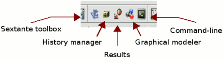
SEXTANTE toolbar
- The SEXTANTE toolbox. The main element of the SEXTANTE GUI, it is used to execute a single algorithm or run a batch process based on that algorithm.
SEXTANTE toolbox
- The SEXTANTE graphical modeler. Several algorithms can be combined graphically using the modeler to define a workflow, creating a single process that involves several sub-processes.
SEXTANTE graphical modeler
- The SEXTANTE command-line interface. Advanced users can use this interface to create small scripts and call SEXTANTE algorithms from them.

SEXTANTE command-line
- The SEXTANTE history manager. All actions performed using any of the aforementioned elements are stored in a history file and can be later easily reproduced using the history manager.

SEXTANTE history manager
- The SEXTANTE results tool. Allows users to search for the generated results during the recent work.
SEXTANTE results
Along the following chapters we will review each one of this elements in detail.
La caja de herramientas de Sextante
Introduction
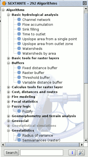
The Toolbox is the main element of the SEXTANTE GUI, and the one that you are more likely to use in your daily work. It shows the list of all available algorithms grouped in different blocks, and is the access point to run them whether as a single process or as a batch process involving several executions of a same algorithm on different sets of inputs.

SEXTANTE toolbox
Depending on the data available in the gvSIG View, you will be able to execute an algorithm or not. When there is enough data for the algorithm to be executed (i.e. the algorithm requires raster layers and you have raster layer already loaded into the View), its name is shown in black, otherwise, it is show in grey.
In the lower part of the toolbox you can find a text box and a search button. To reduce the number of algorithms shown in the toolbox and make it easier to find the one you need, you can enter any word or phrase on the text box and click on the search button. SEXTANTE will search the help files associated to each algorithm and show only those algorithms that include the word or phrase in their corresponding help files. To show all the algorithms again, make a search with an empty string.
To execute an algorithm, just double-click on its name in the toolbox.
Diálogo de algoritmos
Introducción
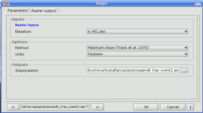
Once you double-click on the name of the algorithm that you want to execute, a dialog similar to the next one is shown (in this case, the dialog corresponds to the Anisotropic cost algorithm).
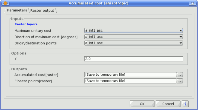
SEXTANTE dialog
This dialog is used to set the input values that the algorithm needs to be executed. There is a main tab named Parameters where input values and configuration parameters are set. This tab has a different content depending on the requirements of the algorithm to be executed, and is created automatically based on those requirements. On the left side, the name of the parameter is shown. On the right side the value of the parameter can be set.
Those algorithms that generate raster layers as output have an additional tab named Raster output. This tab is used to set the characteristics of those output raster layers, specifying its extent and its cell size. On the lower part of the window there is a help button. Click on it to see the context help related to the current algorithm, where you will find detailed description of each parameter and each output generated by the algorithm.
La pestaña de parámetros
Although the number and type of parameters depends on the characteristics of the algorithm, the structure is similar for all of them. The parameters found on the parameters tab can be of one of the following types.
- A raster layer, to select from a list of all the ones available in the View.
- A vector layer, to select from a list of all the ones available in the View.
- A table, to select from a list of all the ones available in the View.
SEXTANTE raster dialog
- A method, to choose from a selection list of possible options.
- A numerical value, to be introduced in a text box.
- A text string, to be introduced in a text box.
- A field, to choose from the attributes table of a vector layer or a single table selected in another parameter.
- A band, to select from the ones of a raster layer selected in another parameter. In both this and the previous type of parameter, the list of possible choices depends on the value selected in the parent parameter.
- A list of elements (whether raster layers, vector ones or tables), to select from the list of the ones available in gvSIG View. To make the selection, click on the small button on the left side of the corresponding row to see a dialog like the following one.
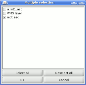
SEXTANTE multiple selection
- A file or folder
- A point, to be introduced as a pair of coordinates in two text boxes (X and Y coordinates)
- A small table to be edited by the user. These are used to defined lookup tables or convolution kernels, among other parameters.
Click on the button on the right side to see the table and edit its values.
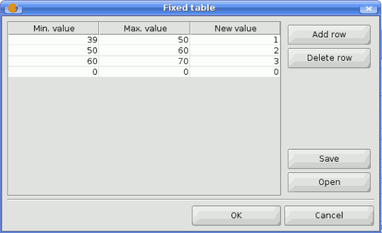
SEXTANTE filter table
Depending on the algorithm, the number of rows can be modified or not, using the buttons on the right side of the window.
La pestaña de salida raster
The Raster output tab is found in those algorithms that generate raster layers. Unlike in most GIS, when combining several raster layers as input for an algorithm, they do not have to have the same extent an cellsize in order to process them together. That is, layers don't have necessarily to match" between them. Instead, the characteristics of the output raster layer are defined and SEXTANTE performs the corresponding resampling and cropping needed to generate layer with those characteristics.
It is responsibility of the user to enter adequate values and be aware of the limitations of this mechanism, so as to generate cartographically correct results. (i.e. you can select a small cell size for the resulting raster layers, but if the input layers you are using have a bad resolution the results will not be geographically sound).
The following options are available in the raster output tab:
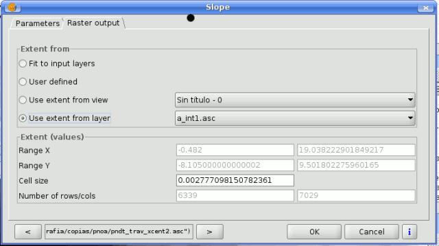
SEXTANTE raster output tab
- Fit to input layers. By default, the characteristics of the output raster layers are set based on the input ones. The minimum extent needed to cover all the input layers is used.
- User defined. The coordinates of the boundaries of the extent and the cellsize are both defined manually, entering the desired values in the corresponding text boxes.
- Use extent from view.. This option will let you use predefined extents from one of the views currently opened.
- Use extent from layer. The extent of a layer can be used as well to define the output characteristics, even if the layer is not used as input to the algorithm. If the selected layer is a vector one, the cellsize will have to be entered manually, since vector layers do not have an associated cellsize.
If an option other than the automatic fitting is selected, SEXTANTE will check that the values are correct and the resulting layers will not be too large (due to, for instance, a wrong cell size). If the output layers seems to large, SEXTANTE will show the next message dialog to ensure that the user really want those layer to be created.
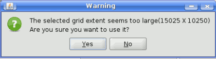
SEXTANTE size warning
Not all algorithms have the first option available, since not all algorithms that generate raster layers take some other raster layer as input. The interpolation algorithms, for instance, take a vector layer and create a raster one. The extent and cellsize of the latter has to be manually defined, since it cannot be set based solely on the input vector layer.
Objetos de datos generados por los algoritmos de Sextante
Data objects generated by SEXTANTE can be of any of the following types:
- A raster layer
- A vector layer
- A table
- A graphical result (chart, graph, etc.)
- A textonly HTML formatted result
Layers and tables can be saved to a file, and the parameters window will contain a text box corresponding to each one of these outputs, where you can type the desired file path. If you do not enter any file path, a temporal file name and folder will be used.
The supported formats for the SEXTANTE cartographic output files are as follows.
- shp
- dxf
- tif
- asc
To select a format, just select the corresponding file extension. If the extension of the file path you entered does not match any of the supported ones, the default extension (the first one in the list of supported ones) will be appended to the file path and the file format corresponding to that extension will be used to save the layer or table.
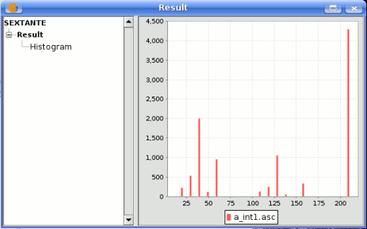
Graphics and texts are kept in memory and shown at the end of the algorithm execution in a new dialog. This dialog will keep the results produced by SEXTANTE during the current session, and can be shown at any time using the Results button. You can save graphical results as images in png format, and texts as HTML files. Rightclick on the name of the result in the tree on the left hand of the window and select Save as....
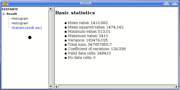
SEXTANTE statistics results
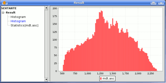
SEXTANTE graphic result
Ayuda contextual
Each SEXTANTE algorithm has its own context help file, which provides detailed information about the meaning of each input parameter and each output object, and gives hints about its usage. To access the context help system, click on the button that you will find in the algorithm dialog, or rightclick on its name on the toolbox and then select See help.
SEXTANTE help icon
The context help system contains not only information about each algorithm, but also description of each one of the elements of the SEXTANTE GUI like the text you are reading now. You will find it at the top of the tree on the left hand side of the help window. Just select an item to see its associated help file on the right canvas.

SEXTANTE help window (NOT AVAILABLE AT THE MOMENT)
Help files associated to each algorithm are stored as XML files, and can be edited using the help authoring tools included with SEXTANTE. Right click on the name of the algorithm in the context help window and select Edit help to get to the following window:

SEXTANTE edit help window (NOT AVAILABLE AT THE MOMENT)
On the left hand side you can select any of the elements to be documented (input parameter and outputs, along with other fixed field such as a general description of the algorithm). Then use the right hand side boxes to enter to text associated to that element or add images.
Modelador gráfico
Introducción
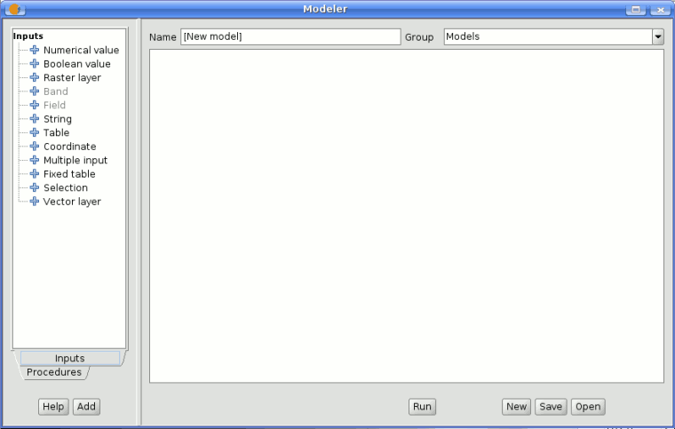
The graphical modeler allows to create complex models using a simple and easytouse interface. When working with a GIS, most analysis operations are not isolated, but part of a chain of operations instead. Using the graphical modeler, that chain of processes can be wrapped into a single process, so it is easier and more convenient to execute than single process later on a different set on inputs. No matter how many steps and different algorithms it involves, a model is executed as a single algorithm, thus saving time and effort, specially for larger models.
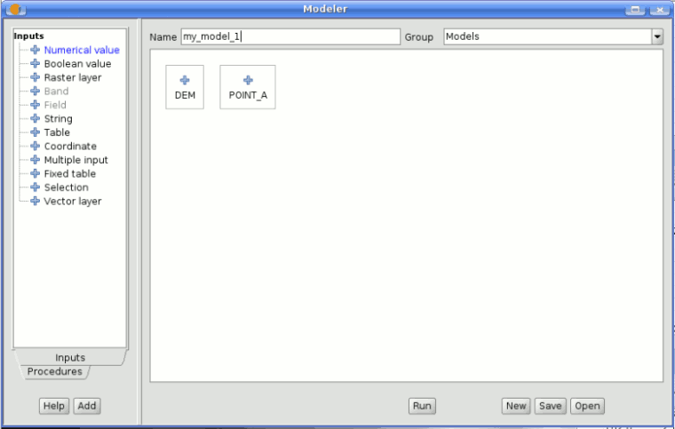
The modeler has a working canvas where the structure of the model and the workflow it represents are shown. On the left part of the window, a panel with two tabs can be used to add new elements to the model.

SEXTANTE modeler window
Creating a model is a two-step process.
- Definition of necessary inputs. These inputs will be added to the parameters window, so the user can set their values when executing the model. The model itself is a SEXTANTE algorithm, so the parameters window is generated automatically as it happens with all the algorithms included in the library.
- Definition of the workflow. Using the input data of the model, the workflow is defined adding algorithms and selecting how they use those inputs or the outputs generated by other algorithms already in the model.
Definición de entradas
The first step to create a model is to define the inputs it needs. The following elements are found in the Inputs tabs on the left side of the modeler window:
- Band
- Raster layer
- Vector layer
- String
- Table field
- Coordinate (Point)
- Table
- Fixed table
- Multiple input
- Selection
- Numerical value
- Boolean value
Double-clicking on any of them, a dialog is shown to define its characteristics. Depending on the parameter itself, the dialog will contain just one basic element (the description, which is what the user will see when executing the model) or more of them. For instance, when adding a numerical value, as can be seen in the next figure, apart from the description of the parameter is needed to set a default value, the type of numerical value and a range of valid values.
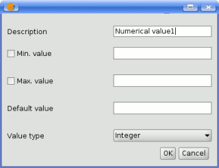
SEXTANTE modeler window for adding values
For each added input, a new element is added to the modeler canvas.
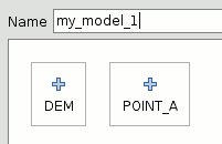
SEXTANTE modeler elements
Definición de procesos
Once the inputs have been defined, it is time to define the algorithms to apply on them. Algorithms can be found in the Processes tab, grouped much in the same way as they are in the toolbox.
SEXTANTE modeler
To add a process, double-click on its name. An execution dialog will appear, with a content similar to the one found execution panel that SEXTANTE shows when executing the algorithm from the toolbox.
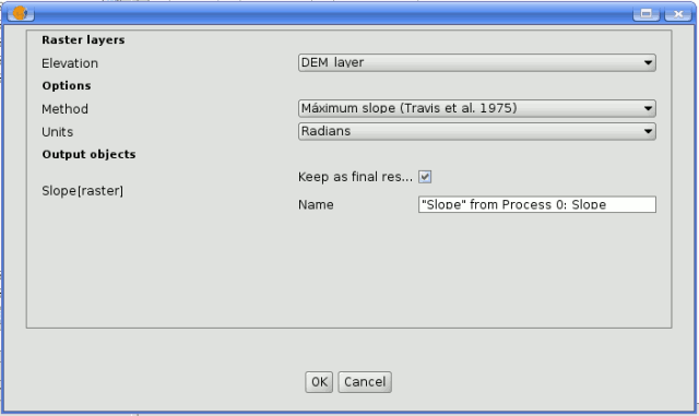
SEXTANTE modeler process
Some differences exist, however, the main one being the absence of a raster ouput tab, even if the selected algorithm generates raster layers as output.
Instead of the textbox that was used to set the filepath for output layers and tables, a checkbox and a text box are found. If the layer generated by the algorithm is just a temporary result that will be used as the input of another algorithm and should not be kept as a final result, the check box should be left unchecked. Checking it means that the result is a final one, and you have to supply also a valid description for the output, which will be the one the user will see when executing the model.
Selecting the value of each parameter is also a bit different, since there are important differences between the context of the modeler and the toolbox one. Let's see how to introduce the values for each type of parameter.
- Layers (raster and vector) and tables. They are selected from a list, but in this case the possible values are not the layers or tables currently loaded in the GIS, but the list of model input or the corresponding type, or other layers or tables generated by algorithms already added to the model.
- Numerical values. Literal values can be introduced directly on the textbox. This textbox is a list that can be used to select any of the numerical value input of the model. In this case, the parameter will take the value introduced by the user when executing the model.
- String. Like in the case of numerical values, literal strings can be typed, or an input string can be selected
- Points. Coordinates cannot be directly introduced. Use the list to select one of the coordinate inputs of the model
- Bands. The number of bands of the parent layer cannot be known at designtime, so it is not possible to show the list of available bands. Instead, a list with band numbers from 1 to 250, as well as the band parameters of the model, is shown. At runtime, SEXTANTE will check if the parent raster layer selected by the user has enough bands and the given band has therefore a valid value, and if not it will generate an error message.
- Table field. Like in the previous case, the elds of the parent table or layer cannot be known at designtime, since they depend of the selection of the user each time the model is executed. To set the value for this parameter, type the name of a field directly in the textbox, or use the list to select a table field input already added to the model. The validity of the selected field will be checked by SEXTANTE at runtime
- Selection. The list contains in this case not only the available option from the algorithm, but also the selection inputs already added to the current model
Once all the parameter have been assigned valid values, click on OK and the algorithm will be added to the canvas. It will be linked to all the other elements in the canvas, whether algorithms or inputs, which provide objects that are used as inputs for that algorithm.
SEXTANTE model
Edición del modelo sobre el lienzo
Once the model has been designed, it can be executed clicking on the Run button. The execution window will have a parameters tab automatically created based on the requirements of the model (the inputs added to it), just like it happens when a simple algorithm is executed. If any of the algorithms of the model generates raster layers, the Raster output tab will be added to the window.
Elements can be dragged to a different position within the canvas, to change the way the module structure is displayed and make it more clear and intuitive. Links between elements are update automatically.
To change the parameters of any of the algorithms of a model, doubleclick on it to access its parameters window.
To delete an element, right-click on it and select Delete. Only those elements that do not have any other one depending on them can be deleted. If you try to delete an element that cannot be deleted, SEXTANTE will show a warning message.
Almacenamiento y recuperación de modelos
Models can be saved to be executed or edited at a later time. Use the Save button to save the current model and the Open model to open any model previously saved. Model are saved in an XML file with the .model extension.
Models saved on the models folder will appear in the toolbox algorithm tree in a group named Models.
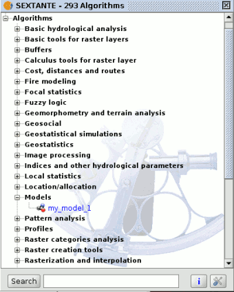
SEXTANTE models on the tree
When the toolbox is invoked, SEXTANTE searches the models folder for files with .model extension and loads the models they contain. Since a model is itself a SEXTANTE algorithm, it can be added to the toolbox just like any other algorithm.
The models folder can be set from the SEXTANTE toolbox, clicking the configuration button at the right lower corner of the window, and then introducing the path to the folder in the corresponding field.
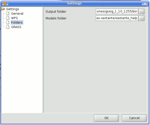
SEXTANTE modeler configuration
Models loaded from the models folder appear not only in the toolbox, but also in the algorithms tree in the Processes tab of the modeler window. That means that you can incorporate a model as a part of a bigger model, just as you add any other algorithm.
Interfaz de procesos batch
Introducción
SEXTANTE algorithms (including models) can be executed as a batch process. That is, they can be executed using not a single set of inputs, but several of them, executing the algorithm as many times as needed. This is useful when processing large amounts of data, since it is not necessary to launch the algorithm many times from the toolbox.
SEXTANTE executing batch
La tabla de parámetros
Executing a batch process is similar to performing a single execution of an algorithm. Parameter values have to be defined, but in this case we need not just a single value for each parameter, but a set of them instead, one for each time the algorithm has to be executed.
Values are introduced using a table like the one shown next.
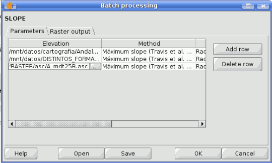
SEXTANTE batch processing
Each line of this table represents a single execution of the algorithm, and each cell contains the value of one of the parameters. It is similar to the parameters tab that you see when executing an algorithm from the toolbox, but with a different arrangement.
By default, the table contains just two rows. You can add or remove rows using the buttons on the right hand side of the window.
Once the size of the table has been set, it has to be filled with the desired values.
Rellenando la tabla de parámetros
Whatever the type of parameter it represents, every cell has a text string as its associated value. Doubleclicking on a cell, this string can be edited, directly typing the desired value. For most of the parameters, however, it is more convenient to use the button on the right hand side of the cell. Clicking on it, a dialog is shown to select the value of the parameter. The content of this dialog depends on the kind of parameter, and it features elements that make it easier to introduce the desired value. For example, for a selection parameter the list of all possible values is shown and the value can be chosen from them.
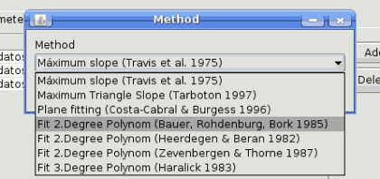
SEXTANTE batch method
For all parameter cells, if the introduced value is correct, it will be shown in black. If the value is wrong (for instance, a numerical value out of the valid range or an option that does not exists for a selection parameter), the text will be shown in red.
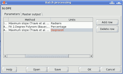
SEXTANTE batch wrong value
The most important different between executing an algorithm from the toolbox and executing it as part of a batch process is that input data objects are taken directly from files, and not from the set of layers already opened in the GIS. For this reason, any algorithm can be executed as a batch process even if no data objects at all are opened and the algorithm cannot be called from the toolbox.
Filenames for input data objects are introduced directly typing or, more conveniently, clicking on the button on the right hand of the cell, which shows a typical file chooser dialog. Multiple files can be selected at once. If the input parameter represents a single data object and several files are selected, each one of them will be put in a separate row, adding new ones if needed. If it represents a multiple input, all the selected files will be added to a single cell, separated by commas.
If multiple bands are required, a more complex dialog is shown, which incorporates a table for selecting both layer files and bands. Click on the cells on the left side to select the file which contains the raster layer. Then click on the left side to select the bands you want to use from that layer. To know the number of bands in a layer it would be necessary to open it. However, SEXTANTE does not open the layer, and shows instead a list of bands from 1 to 250 to select from. If you select a band that does not exist in the selected layer, an error message will be shown at execution time.
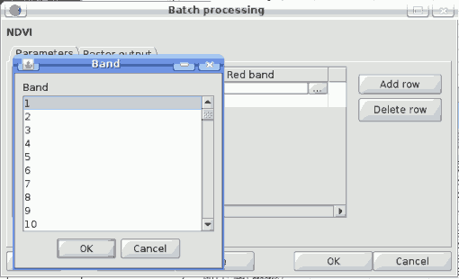
SEXTANTE batch band dialog
Output data objects are always saved to a file and, unlike when executing an algorithm from the toolbox, saving to a temporary one is not permitted. You can type the name directly or use the file chooser dialog that appears when clicking on the accompanying button. This dialog differs slightly from the standard one, incorporating some additional fields for autocompletion.
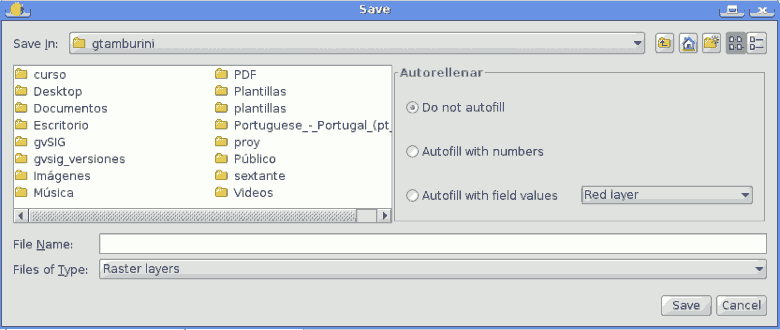
SEXTANTE batch save dialog
If the default value (Do not autofill) is selected, SEXTANTE will just put the selected filename in the selected cell from the parameters table. If any of the other options is selected, all the cells below the selected one will be automatically lled based on a defined criteria. This way, it is much easier to ll the table, and the batch process can be defined with less effort.
Automatic filling can be done simply adding correlative numbers to the selected filepath, or appending the value of another field at the same row. This is particularly useful for naming output data object according to input ones. Cells can be selected just clicking and dragging. Selected cells can be copied and pasted in a different place of the parameters table, making it easy to ll it with repeated values.
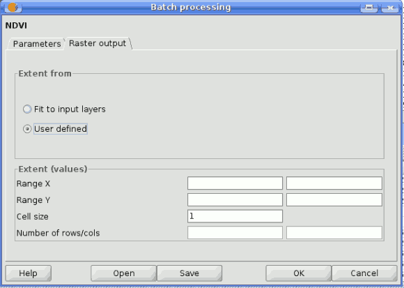
Estableciendo las características de las salidas raster
Just like when executing a single algorithm, when running a batch process that generates raster layers you must define the extent and cellsize of the raster layers to be created. The corresponding Raster Output tab is similar to the one found when running a single algorithm, but only contains two options: t to input layers and user-defined.
The selection will be applied to all the single executions contained in the current batch process. If you want to use different raster output configurations, then you must define different batch processes.
SEXTANTE batch raster output dialog
Ejecutando el proceso por lotes
To execute the batch process once you have introduced all the necessary values, just click on OK. SEXTANTE will show the progress of each executed algorithm, and at the end will show a dialog with information about the values used and the problems encountered during the execution of the whole process.
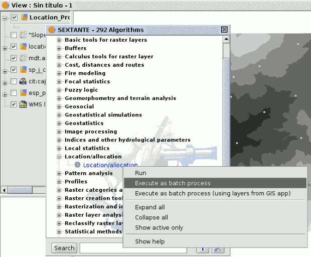
Procesos por lotes con capas ya cargadas
It is possible to execute the batch processing from a set of layers from the current view, clicking on the correct option in the toolbox tree, similar as it was the usual batch processing.
Interface de línea de comandos
Introducción
The command-line interface allows advanced users to increase their productivity and perform complex operations that cannot be performed using any of the other elements of the SEXTANTE GUI. Models involving several algorithms can be defined using the command-line interface, and additional operations such as loops and conditional sentences can be added to create more flexible and powerful workflows.
La interfaz
Introducción
Invoking the command-line interface will make the following dialog appear.

SEXTANTE command-line
The SEXTANTE command-line interface is based on BeanShell. BeanShell is a Java source interpreter with object scripting language features, that meaning that it dynamically executes standard Java syntax and extends it with common scripting conveniences such as loose types, commands, and method closures like those in Perl and JavaScript.
A detailed description of BeanShell and its usage can be found at the BeanShell website. Refer to it if you want to learn more about generic BeanShell features. This chapter covers only those particular elements which are related to SEXTANTE geoalgorithms.
By using the extension mechanisms of BeanShell, SEXTANTE adds several new commands to it, so you can run geoalgorithms or get information about the geospatial data you are using, among other things.
Java users can create small scripts and programs combining standard elements of Java with SEXTANTE commands. However, those who are not familiar with Java can also use the command-line interface to execute single processes or small sets of them, simply calling the corresponding methods.
A detailed description of all SEXTANTE commands is given next.
Obtener información sobre los datos
Algorithms need data to run. Layers and tables are identified using the name they have in the table of contents of the GIS (and which usually can be modied using GIS tool). To call a geoalgorithm you have to pass it an identifier which represents the data to use for an input.
The data() command prints a list of all data objects available to be used, along with the particular name of each one (i.e. the one you have to use to refer to it). Calling it you will get something like this:
RASTER LAYERS
-----------------
mdt25.asc

VECTOR LAYERS
-----------------
Curvas de nivel

TABLES
-----------------
Be aware that gvSIG allows you to have several layers with the same name. SEXTANTE will just take the first one which matches the specified identifier, so you should make sure you rename your data object so each one of them has a unique name.
To get more information about a particular data object, use the describe(name of data object) command. Here are a few examples of the result you will get when using it to get more information about a vector layer, a raster layer and a table.
>describe points
Type: Vector layer - Point
Number of entities: 300
Table fields: | ID | X | Y | SAND | SILT | CLAY | SOILTYPE | EXTRAPOLAT |

>describe dem25
Type: Raster layer
X min: 262846.525725
X max: 277871.525725
Y min: 4454025.0
Y max: 4464275.0
Cellsize X: 25.0
Cellsize Y: 0.0
Rows: 410
Cols: 601

>describe spatialCorrelation
Type: TableNumber of records: 156
Table fields: | Distance | I_Moran | c_Geary | Semivariance |
Obtener información sobre los algoritmos de análisis geográfico
Once you know which data you have, it is time to know which algorithms are available and how to use them.
When you execute an algorithm using the toolbox, you use a parameters window with several fields, each one of them corresponding to a single parameter. When you use the command line interface, you must know which parameters are needed, so as to pass the right values to use to the method that runs that algorithm. Of course you do not have to memorize the requirements of all the algorithms, since SEXTANTE has a method to describe an algorithm in detail. But before we see that method, let's have a look at another one, the algs() method. It has no parameters, and it just prints a list of all the available algorithms. Here is a little part of that list as you will see it in your command-line shell.
bsh % algs();
acccost-------------------------------: Accumulated cost(isotropic)
acccostanisotropic--------------------: Accumulated cost (anisotropic)
acccostcombined-----------------------: Accumulated cost (combined)
accflow-------------------------------: Flow accumulation
acv-----------------------------------: Anisotropic coefficient of variation
addeventtheme-------------------------: Points layer from table
aggregate-----------------------------: Aggregate
aggregationindex----------------------: Aggregation index
ahp-----------------------------------: Analytical Hierarchy Process (AHP)
aspect--------------------------------: Aspect
buffer--------------------------------: Buffer
On the right you find the name of the algorithm in the current language, which is the same name that identifies the algorithm in the toolbox. However, this name is not constant, since it depends on the current language, and thus cannot be used to call the algorithm. Instead, a command-line is needed. On the left side of the list you will find the command-line name of each algorithm. This is the one you have to use to make a reference to the algorithm you want to use.
Now, let's see how to get a list of the parameters that an algorithms require and the outputs that it will generate. To do it, you can use the describealg(name of the algorithm) method. Use the command-line name of the algorithm, not the full descriptive name.
For example, if we want to calculate a ow accumulation layer from a DEM, we will need to execute the corresponding module, which, according to the list show using the ags() method,is identified as accflow. The following is a description of its inputs and outputs.
>describealg("accflow")
Usage: accflow(DEM[Raster Layer]
              WEIGHTS[Optional Raster Layer]
              METHOD[Selection]
              CONVERGENCE[Numerical Value]
              FLOWACC [output raster layer])
Ejecutando algoritmos
Now you know how to describe data and algorithms, so you have everything you need to run any algorithm. There is only one single command to execute algorithms: runalg. Its syntax is as follows:
> runalgname_of_the_algorithm, param1, param2, ..., paramN)
The list of parameters to add depends on the algorithm you want to run, and is exactly the list that the describealg method gives you, in the same order as shown.
Depending on the type of parameter, values are introduced differently. The next one is aquick review of how to introduce values for each type of input parameter
- [Raster Layer], [Vector Layer]o [Table]. Simply introduce the name that identies the data object to use. If the input is optional and you do not want to use any data object, write #".
- [Numerical value]. Directly type the value to use or the name of a variable containing that value.
- [Selection]. Type the number that identies the desired option, as shown by the options command
- [String]. Directly type the string to use or the name of a variable containing it.
- [Boolean]. Type whether true" or false" (including quotes)
- [Multiple selection - tipo datos]. Type the list of objects to use, separated by commas and enclosed between quotes.
For example, for the maxvaluegrid algorithm:
Usage: runalg("maxvaluegrid",
      INPUT[Multiple Input - Raster Layer]
      NODATA[Boolean],
      RESULT[Output raster layer])
The next line shows a valid usage example:
> runalg("maxvaluegrid", "lyr1, lyr2, lyr3", "false", "#")
Of course, lyr1, lyr2 and lyr3 must be valid layers already loaded into gvSIG.
When the multiple input is comprised of raster bands, each element is represented by a pair of values (layer, band). For example, for the cluster algorithm:
Usage: runalg ("cluster",
      INPUT[Multiple Input - Band]
      NUMCLASS[Numerical Value]) ***************
The next line shows a valid usage example:
> runalg("cluster, "lyr1, 1, lyr1, 2, lyr2, 2", 5, "#", "#")
The algorithm will use three bands, two of them from lyr1 (the first and the second ones of that layer) and one from lyr2 (its second band).
- [Table Field from XXX ]. Write the name of the field to use. This parameter is case sensitive.
- [Fixed Table ]. Type the list of all table values separated by commas and enclosed between quotes. Values start on the upper row and go from left to right. Here is an example:
runalg("kernelfilter", mdt25.asc, "-1, -1, -1, -1, 9, -1, -1, -1, -1", "#")
- [Point ]. Write the pair of coordinates separated by commas and enclosed between quotes. For instance "220345, 4453616"
Input parameters such as strings or numerical values have default values. To use them, type "#" in the corresponding parameter entry instead of a value expression.
For output data objects, type the filepath to be used to save it, just as it is done from the toolbox. If you want to save the result to a temporary file, type "#".
Ajustar las características de la capa raster de salida
Just like when you execute a geoalgorithm from the toolbox, when it generates new raster layers you have to define the extent and cellsize of those layers.
By default, those characteristics are defined based on the input layers. You can toggle this behaviour using the autoextent command.
> autoextent("true"/"false)
If you want to define the output raster characteristics manually or using a supporting layer, you have to use the extent command, which has three different variants.
Usage: extent(raster layer[string])
       extent(vector layer[string], cellsize[double])
       extent(x min[double], y min[double],
              x max[double], y max[double],
              cell size[double])
Type "autoextent" to use automatic extent fitting when possible
When this command is used, the autoextent functionality is automatically deactivated.
El historial de procesos
Introducción
Every time you execute a SEXTANTE algorithm, information about the process is stored in the SEXTANTE history manager. Along with the parameters used, the date and time of the execution are also saved.
This way, it is easy to track the and control all the work that has been developed using SEXTANTE, and easily reproduce it.
The SEXTANTE history manager is a set of registries grouped according to their date of execution, making it easier to find information about an algorithm executed at any particular moment.
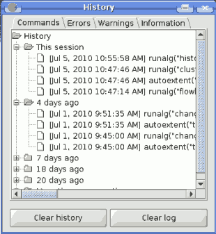
SEXTANTE history manager
Process information is kept as a command-line expression, even if the algorithm was launched from the toolbox. This makes it also useful for those learning how to use the command-line interface, since they can call an algorithm using the toolbox and then check the history manager to see how that same algorithm could be called from the command-line.
Apart from browsing the entries in the registry, processes can be reexecuted, simply double-clicking on the corresponding entry.
-----------------------------------
- Se ha producido un error en el documento Navegación , accediendo a la imagen picture_22.png, que probablemente no existe. Se han encontrado las siguientas alternativas [1, 2, 3, 4, ]
- Se ha producido un error en el documento Navegación , accediendo a la imagen picture_14.png, que probablemente no existe. Se han encontrado las siguientas alternativas [1, 2, 3, 4, ]
- Se ha producido un error en el documento Ayuda contextual , accediendo a la imagen stnt_help.png, que probablemente no existe. No se han encontrado alternativas
- Se ha producido un error en el documento Ayuda contextual , accediendo a la imagen stnt_edit_help.png, que probablemente no existe. No se han encontrado alternativas


