- Raster
- Teledetección
- Clasificación de un ráster
- Cálculo de Bandas
- Descripción de la calculadora de bandas
- Realizar un cálculo
- Opciones de salida
- Salvar y cargar expresiones
- Definición de regiones de interés
- Perfiles de imagen
- Árboles de decisión
- Funciones de Transformación Multiespectral
- Fusión de Imágenes
- Funcionalidades de capa
- Apertura de formatos
- Carga de capas RAW
- Estadísticas básicas
- Filtrado
- Histograma
- Información de la capa
- Rango de escalas
- Realce (Propiedades)
- Salvar a raster
- Realces Radiométricos
- Salvar Como
- Recorte de capas
- Reproyección
- Seleccionar Capas Raster
- Tablas de color y gradientes
- Selector de bandas y ficheros
- Transparencia por pixel y opacidad
- Valores NoData
- Zoom a la resolución del raster
- Vectorización automática
- Vista de análisis
- Componentes generales
- Vista previa
- Selector de resultados
- Control de tablas
- Barra de progreso
- Estadísticas finales de generación de capa
- Barra de herramientas desplegable
- Transformaciones geográficas
Raster
Teledetección
Clasificación de un ráster
Clasificación supervisada
Descripción funcionalidad
The main objectif of classifying an image according to previously established parameters is one of the most common goal of the remote sensing users. This tool allows to obtain classified maps derived from remote sensing data.
Thus the final goal is to produce a single band image, having same size and characteristiques of the original one, with the difference that single pixel value is a label identifying the category, among the selected ones, to which the pixel has been assigned during the classification procedure.
Clasificación supervisada de un ráster en gvSIG
gvSIG allows to perform a raster supervised classification by three different methods: maximum likelihood, minimum distance and parallelepiped.
To open the classification tool, you have to use the remote sensing toolbar by selecting “Raster process” from the left button and “Classification” from the right button.

The following window will be displayed
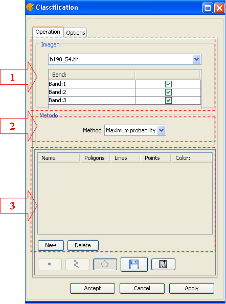
Operations Panel
In (1) choose the raster to classify. You can choose only an image already loaded in the view. For the selected image, chose also the bands you use to perform the classification process.
In (2) choose the method you use to perform the classification, you can select between: maximum likelihood, minimum distance and parallelepiped.
In (3) edit the classes on which the classification will be performed. By default, when you select the image to classify, a number of classes equal to the number of regions of interest (ROIs) linked to image are loaded.
You can modify (see document of ROIs editing) class number and composition, according to your need, without modifying the original ROIs.
Options Panel
To setup the parameters and the output options, activate the Option panel
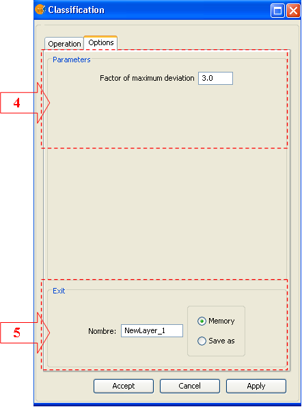
In (4) adjust the maximum standard deviation if the selected method is the parallelepiped one. In case of other methods, the panel will be empty.
In (5) setup the usual output parameters. Choose the output file name and path.
Cálculo de Bandas
Descripción de la calculadora de bandas
Band calculator allows you to perform mathematical operations between band values of the same image or from different images maintaining some spatial constraints (always on original values). The result of this operation is a one-band raster image.
To open the Calculator tool, you have to use the remote sensing toolbar by selecting “Raster process” from the left button and “Raster calculator” from the right button.
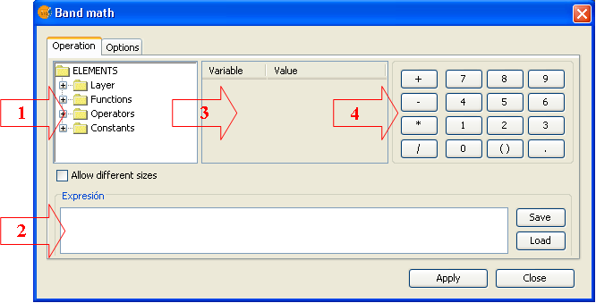
- the elements tree: allows to add different elements to the operation just browsing and double click over the selected element.
- expression frame: expression used for the operation
- table of variables: will contain the relation between variables and bands
- calculator keyboard: allow to insert numerical values as well as basic operators in the expression.
Realizar un cálculo
To perform a calculation among bands, you have to introduce an expression in the expression frame and link one band of the raster layers loaded in the TOC to one of the variables listed in the expression.
Write the expression in the expression frame. To do that, you can use all the elements of the calculator.
The decision tree contains the raster layer bands, functions, operators and constants that can be used to compose the expression. Make double click on the chosen element to introduce it in the expression (in the position where the cursor is located). For the bands, you will introduce a varaible that will be automatically associated to the band in the variables table.
Use the keyboard of the calculator to introduce numbers, operators, parenthesis and decimal separator in the expression.
In the variables table you can establish the association between the variables present in the expression and the bands of the raster layer. To link one band to one variable, or to change a link, select the table and double click over the desired band in the decision tree.
Check the box “Allow different dimensions” if you want that the bands having different dimensions, position or pixel size will be part of the calculation. This option involve the use of interpolation to obtain a result.
The result of a calculation is a one band raster layer, of type double, that contain the result of the expression for the pixels presents in ALL the input bands and the “no-data” value for the others.
Opciones de salida
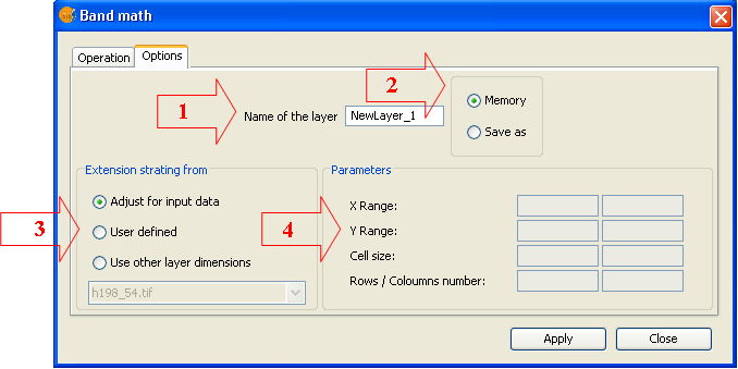
In this window you can select the options for the generation of the calculus result.
Name of the layer (1): Introduce the name of the raster layer that will be loaded in the window as calculus result.
Destination of the result (2): Select if you prefer to save the result as a file or to keep in memory. In the first case you will be asked for the path and the name of the file as the calculation will start. If you choose to keep in memory, you can save it later trough the option “Save as” by clicking with the right mouse button over the corresponding layer in the TOC.
Extension of the resulting raster (3). You can choose the extension and the cell size from the following possibilities:
1. Adjust to the input data: The extension of the resulting raster layer will be the union of the single band extensions presents in the calculation. The resulting cell size will be the smaller one amongst the bands presents in the calculation.
2. User defined: Use this option to introduce in the frame Parameters (4) maximum and minimum X and Y values and the output cell size.
3. Use other layer extension: The extension of the resulting layer will assume the ones of the selected raster layer.
Salvar y cargar expresiones
Click the button Save of the main control panel of the band calculator to save the expression shown in the Expression frame. A dialog window will appear to input the path and the name of the output file.
Click the button Load of the main control panel of the band calculator to an expression previously saved. The expression has to be saved as .exp
Definición de regiones de interés
Descripción de Herramienta edición Rois
This tool allows defining Regions of Interest (ROIs) over one raster layer. These regions or areas of interest can be used to derive statistics, classification processes, creation of masks or other applications.
To launch the ROIs edit tool for one layer you have to use the remote sensing toolbar by selecting “Raster layer” from the left button and “Area of interest” from the right button. You have to check that in the scrolling text window, the layer over which you want to draw the ROIs is selected.

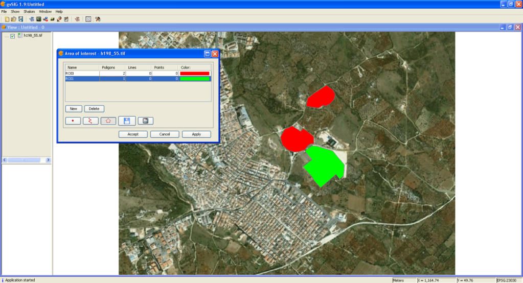
The following window allows defining new ROIs linked to the selected layer.
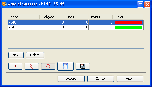
ROI definition step by step
Click over New. A new entry line corresponding to the new ROI will appear in the table. By default, new ROI does not contain any geometry.
Select the geometry you want for the new ROI by activating the corresponding control.
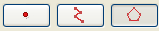
1- The first control allows to add a point to the selected ROI.
2- The second one a linear geometry.
3- The last one a polygon geometry.
Once selected the tool, draw the selected geometry aver the layer.
Add geometries over an already existing ROI
To add a new geometry to a ROI, select the corresponding ROI in the table.
Activate the corresponding control according to the geometry to add
Once drawn the geometry on the view, the ROI will be updated.
Delete a ROI
To delete a ROI select the corresponding line in the table.
Once selected the ROI, click on Delete.
Save a ROI as a shapefile
This option allows to export defined ROIs into a shapefile. The fields of this shapefile will be: (ROI name), R (R value in RGB), G (G value in RGB), and B (B value in RGB).
For each type of geometry linked to the selected ROIs, a Polygon, Polyline or Point file will be created that will manage the corresponding geometries of all the ROIs defined in the table.
Load ROIs from a shapefile
This option allows loading in the ROI tool regions defined by a shapefile. It is compulsory that the shapefile has the fields name, R, G, B. Additional fields can be present as well. Once loaded the ROI, it can be edited in the same way of any other ROI created with the ROI edit tool.
Perfiles de imagen
Descripción Herramienta de Perfiles
This tool allows visualising as a graphic the spectral profile of one point of the image (Z Profile) or the profile of a series of pixel belonging to a path drawn by the user.
To open the Profiles visualization tool, you have to use the remote sensing toolbar by selecting “Raster layer” from the left button and “Image profile” from the right button. You have to check that in the scrolling text window, the layer over which you want to visualize the profiles is selected.

The following window allows to define profiles over the layer.
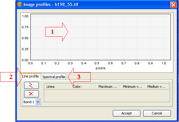
- Area over which you the graphic corresponding to the created profiles is drawn.
- Line profile. Panel to edit and visualize path profiles.
- Spectral profile. Panel to edit and visualize points spectral profiles.
Line profile
The panel to manage the line profiles disposes, in addition to the table, of the following controls

Add a new profile to the table. Once activated the control you draw the desired path over the view.

Delete the selected profile in the table by deleting the linked geometry and the graphic.

Select the band for which the profile will be created.
Spectral profile
The panel to manage point profiles has the following additional controls.

Add a new profile to the table. By control activation you choose the point on the image.
Delete the profile selected in the table by deleting the linked geometry and the graphic.
Árboles de decisión
Descripción funcionalidad de árboles de decisión
Decision trees are used to represent and classify a list of conditions that can occur one after the other in order to obtain a classification of image pixel values.
To open the Decision tree tool, you have to use the remote sensing toolbar by selecting “Raster proces” from the left button and “Decision tree” from the right button.

Decision tree tool will appears as follow.
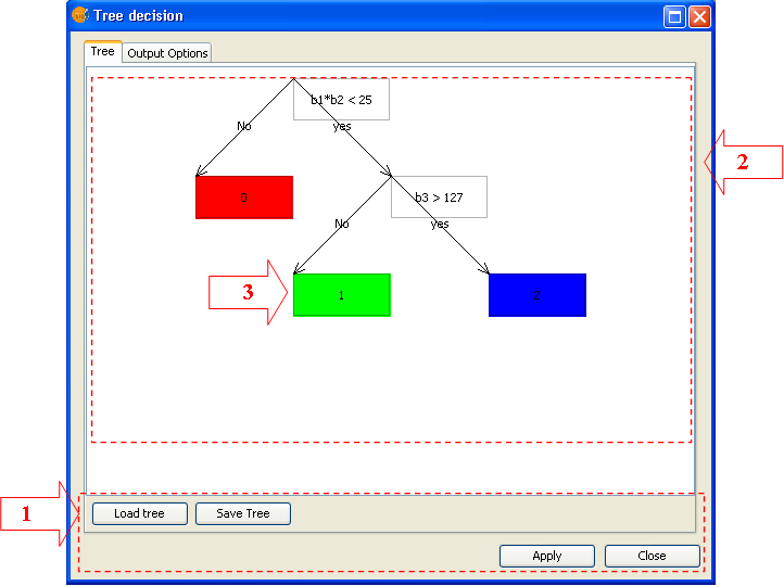
Description of the basic elements
- Menu.
From the Tree panel you can save or load a decision tree. By clicking on Close, you close the entire tool.
- Editing Decision tree panel.
On this panel you draw all the nodes that will affect the final tree configuration.
- Condition Nodes
To set up the tree, it is necessary to add and edit the decision nodes. Decision nodes are the ones appearing in colour in the panel. These nodes are linked to a Boolean expression whose evaluation, for each element of the selected variables, will lead to a result node or to a new evaluation node.
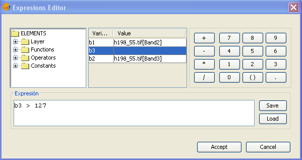
To add a new Condition Node it is necessary to click with the mouse right button (addChild) over a Result Node that you want to split. To assign the evaluation expression to the corresponding node, double click on the node and setup the condition by the expression editor that is shown in the following figure.
- Result Nodes or Leaf Nodes.
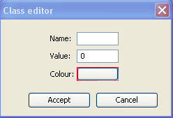
Each Decision Node has to two linked Leaf Nodes corresponding to positive or negative evaluation of the condition. These nodes appear coloured in the panel. They correspond to the assigned colour and value assigned in the result. These values can be modified from the window shown in the following figure and that can be activated by double click over the node.
Execution Options
Once edited the tree corresponding to the desired conditions, you can choose for a full execution or, on the contrary, for a partial execution starting from a given Condition Nodes. To perform the second option, it is necessary to activate the node contextual menu (right mouse button) and select ejecutar.
Output options
In the output options panel you can setup the parameters for the output raster.
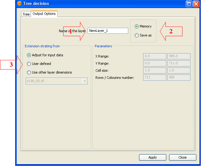
- File name
- Result file path: Select if you want to save the result as a file or to keep in Memory. In the first case you will be asked to specify the destination folder and the file name before launching the calculation. If you choose to keep in memory, you will be able to save it later by the option “Save as” by clicking with the right mouse button over the corresponding layer in the TOC.
- Extension of resulting raster. You can choose result dimension and pixel size as follow:
Adjust from input data: the raster dimension will consider pixel size of all the bands involved in the calculation. Smallest pixel size will be adopted as result.
User defined: Choose this option to input X and Y minimum and maximum values as well as resulting pixel size.
Use other layer dimensions: output raster dimension will assume the parameters of the selected raster layer
Funciones de Transformación Multiespectral
Descripción Funcionalidad de Componentes Principales
The principal components analysis is a multispectral transformation that whose goal is to avoid the use of redounding information in image bands. This technique allows transforming a list of bands into new variables called interlinked variables, absorbing most of data variability in an initial bands subset.
To open the Principal Components tool, you have to use the remote sensing toolbar by selecting “Raster process” from the left button and “Multispectral transformation” from the right button.

The dialog window will appears as follow.
Step by step procedure to perform the transformation
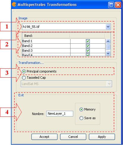
- From the combo box, chose the image to which the transformation will be applied (1).
- Select the bands involved in the process in (2)
- Choose the Principal Components option. (3)
- Select output options. Select if you want to save the result as a file or to keep in Memory. In the first case you will be asked to specify the destination folder and the file name before launching the operation. If you choose to keep in memory, you will be able to save it later by the option “Save as” by clicking with the right mouse button over the corresponding layer in the TOC.
Start the process by Apply or Accept.
Later on, and during the analysis procedure, a dialog window similar to the one in the following figure will appear.
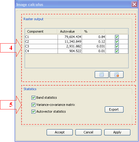
- Table fo components selection In this table you collect the information linked to every component calculated by the bands selected in the first window. The table include information of the corresponding autovalue and the percentage of variability absorbed by the component related to the total variability. The resulting image will be obtained according to the selected components
- Process statistics. The statistics generated in the previous procedure can be exported into a text file. To do this, every checkbox corresponding to the parameters must be selected, click on the option Export and select the path of the output file.
The image creation start by click on Apply or Accept. The result is a float image with as many bands as the selected components and it will automatically load in the view as the process finishes.
Descripción de Transformación Tasseled Cap
Tasseled Cap transformation aims to detect relevant spectral characteristics of developing vegetation surface, with the main goal to detect specific culture by the use of spectral ranges of multitemporal Landsat Images.
To open the Tasseled Cap tool, you have to use the remote sensing toolbar by selecting “Raster process” from the left button and “Multispectral transformation” from the right button.
The dialog window will appear as follow.
Step by step procedure to perform the transformation
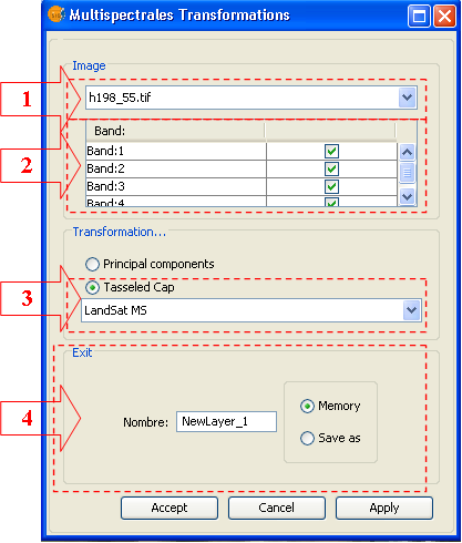
- From the combo box, chose the image to which the transformation will be applied (1).
- Select the bands involved in the process in (2) The number of selected bands is strictly related to the transformation type that will be applied. Thus, for MS transformation 4 bands are needed while for TM and ETM, 6 bands. In the case of the band numbers does not fit transformation needs, the user will be informed.
- In the scroll menu choose the transformation type after having checked the Tasseled Cap checkbox. Transformation types are LandSat MS, LandSatTM and LandSat ETM+.
- Select output options. Select if you want to save the result as a file or to keep in Memory. In the first case you will be asked to specify the destination folder and the file name before launching the operation. If you choose to keep in memory, you will be able to save it later by the option “Save as” by clicking with the right mouse button over the corresponding layer in the TOC.
Start the process by Apply or Accept.
The result is a float image with as many bands as the selected components and it will automatically load in the view as the process finishes
Fusión de Imágenes
Descripción de funcionalidad de fusión de imágenes
The technique of combining images having different spectral or spatial resolution is called image fusion. The goal is to increment the resolution of images having a low spatial resolution using the corresponding panchromatic image. The result is a multispectral image having a resolution close to the panchromatic one.
To open the Image Fusion tool, you have to use the remote sensing toolbar by selecting “Raster process” from the left button and “Images fusion” from the right button.

The dialog window will appear as follow.
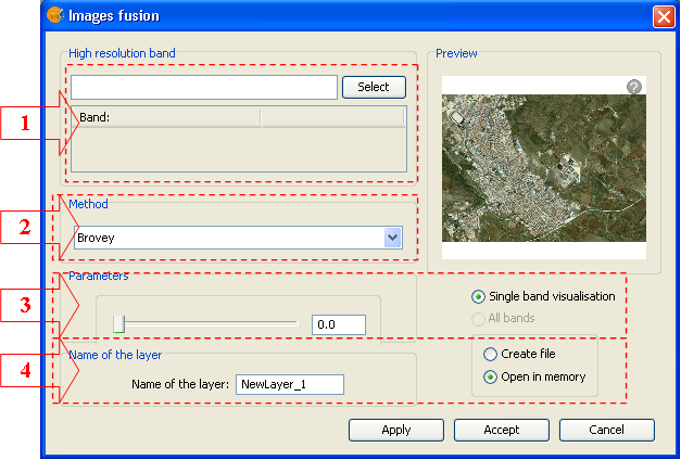
Description of the basic elements
- Panel to select the high resolution band
Using the button Select, chose the image or panchromatic band that will be used in the process.
- Panel to select the fusion method
- In this panel you select the fusion method. You can choose between :
- Brovey
- IHS
- Principal Components
- Wavelets
- Parameters Panel
In this panel you can setup the parameters of any single method listed in (2).
- Options panel
Output options include the possibility to name the output file as well as the usual management options. The result can be obtained just for the visualised bands as well as for all the raster bands.
Funcionalidades de capa
Apertura de formatos
Descripción
You can add layers from disk files by selecting the option "Add Layer" and click on the "Add" button. A file browser window appears. Choose the "gvSIG Raster Driver" option from the "Files of type" pull-down menu. Now, all supported raster file types located in the directory will be shown. You can select one or more of the files to open.
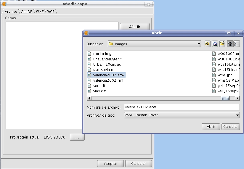
Add Layer Dialog and file browser window with the image driver
Files with the following extensions are supported:
- "Ecw"
- "sid"
- "bmp" of Microsoft
- "gif" Graphics Interchange Format
- "tif" TIFF format
- "tiff" TIFF format with 4-char extension
- "jpg" JPEG format
- "jp2" JPG200 format
- "jpeg" JPEG format with 4-char extension
- "png" Portable Network Graphics
- "vrt" GDAL Virtual Format
- "dat" of Envi
- "lan" of Erdas
- "gis" of Erdas
- "img" of Erdas
- "pix" of PCI Geomatics
- "aux" of PCI Geomatics
- "adf" of ESRI
- "mpr" of Ilwis
- "mpl" of Ilwis
- "asc" ascii grid of ArcInfo
- "pgm", PNM grayscale files
- "ppm", PNM files in RGB
- "rst" of IDRISI
- "rmf" Raster Matrix Format. This format has nothing to do with gvSIG's Raster Metafile, which cannot be loaded as raster file.
- "kap" Nautical Chart Format
- "hdr" Esri hdr
- "raw" RAW format
- "nos"
In addition, only on Linux, it is possible to open GRASS raster layers. This format requires a valid directory structure.
With certain formats, additional dialogs that prompt for parameters or options may appear before the layer is loaded, as for example:
- Introduction of headers for RAW files.
- Introduction of georeferencing if needed.
- Projection parameters.
These options will be explained in the corresponding sections.
Carga de capas RAW
Descripción
gvSIG supports RAW images but before these can be loaded, users will be prompted for the necessary parameters.
To open a RAW image, select the option "Add layer" from the View menu or the corresponding button from the view toolbar. Click on "Add" and select the .RAW image to open. Choose the "gvSIG Raster Driver" option from the "Files of type" pull-down menu.
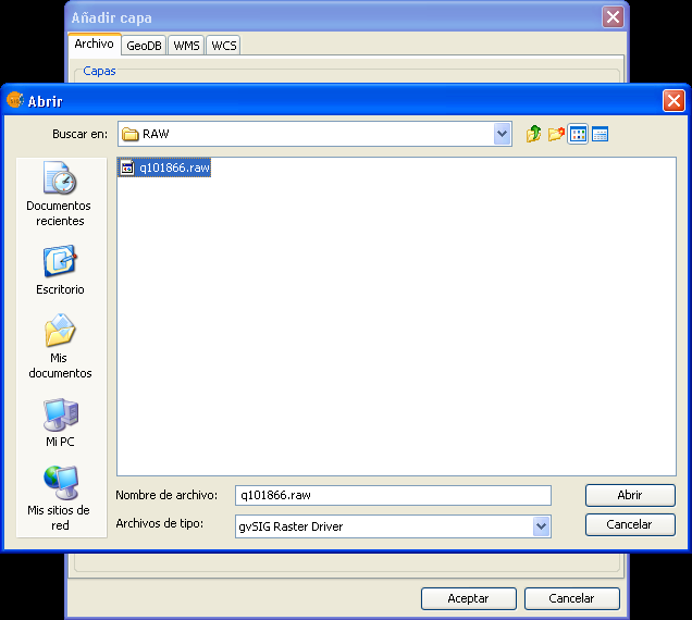
Loading .raw images
When opening the selected file, the following dialog window prompts for the RAW image parameters:
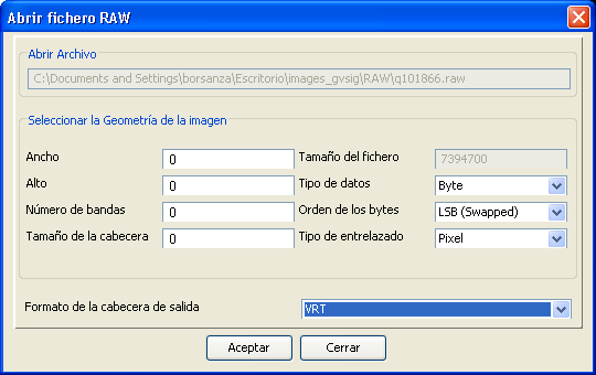
Configuration dialog for image parameters
RAW images basically consist of a continuous string of numbers without a header or other information. Therefore, users will need to supply the information through this dialog. To open a .RAW image you need to have writing permissions to the directory where the image is located.
The following parameters should be provided:
- Width: Image width in pixels.
- Height: Image height in pixels.
- Number of bands: Total number of bands in the image.
- Header size: This parameter is optional and can be omitted if unknown.
- File size: This field is filled automatically when the file is selected.
- Data type: Data type of the image. You need to select one data type from the list.
- Byte order: The order of the bytes in the image (LSB, MSB)
- Band interleaving: the way that the data is stored in the image: by pixel, by band or by line.
After completing the dialog, a header file VRT is created from the supplied parameters. The header file is written in XML format and will be saved with a VRT extension in the same data directory. If some of the parameters are unknown, the layer cannot be displayed correctly. The next time when you are loading the same .RAW file, you do not need to re-enter the parameters if you choose the "gvSIG Raster Driver" and select the VRT file with the stored parameters. However, if you want to load the image with different parameters, you need to load the RAW file again and follow the same procedure, which will overwrite the VRT file with the new parameters.
Estadísticas básicas
Descripción
gvSIG can generate basic statistics over raster layers, which you can access through the option "Raster properties" that opens a dialog window with multiple tabs containing information about the selected raster layer. Select the "General" tab to see the layer statistics.
The dialog window "Raster properties" can be accessed in two ways: by right-clicking the raster layer in the table of contents, or from the raster properties icon in the toolbar:

Raster Properties icon
In this tab, you can see the layer statistics grouped by band. For each band the following information is shown:
- Minimum: Minimum value in the band.
- Maximum: Maximum value in the band.
- RGB Minimum: Minimum RGB value in the band.
- RGB Maximum: Maximum RGB value in the band.
- Mean: The average of all the values in the band.
- Variance: The amount of variation within the values in the band.
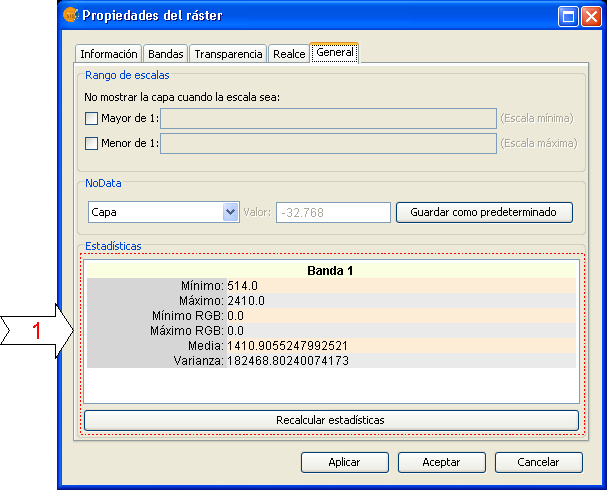
Raster properties window with image statistics
In case that the statistics are incomplete or erroneous, you can use the option "recalculate statistics" to regenerate the statistics.
Filtrado
Descripción
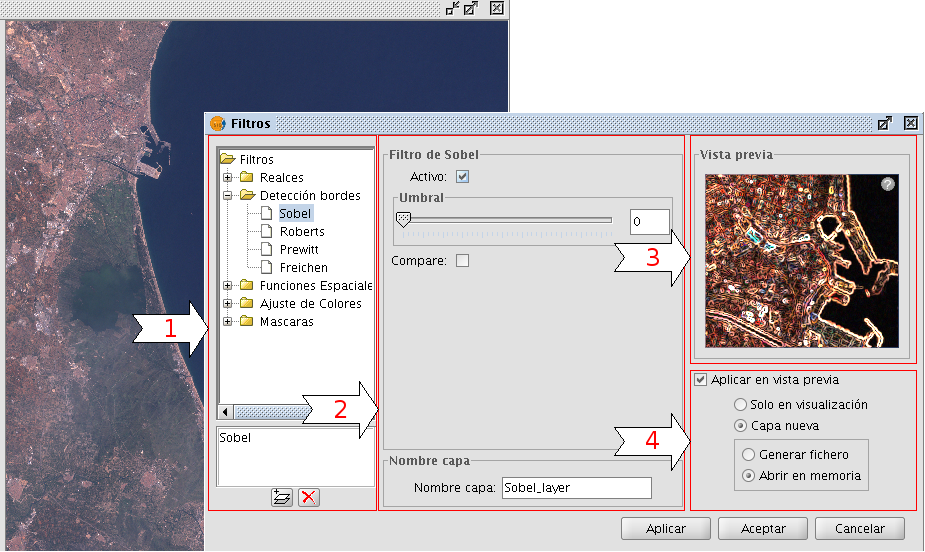
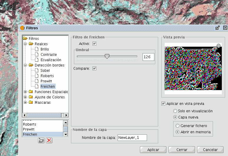
Filtering is a process by which we can enhance images. gvSIG can filter images through a variety of filtering methods. In the upper left part of the Filter dialog, the filters are grouped by type (1). By double-clicking one of the filters or by clicking on the "Add Filter" button on the bottom left, the filter will be added to the list of filters in the lower left part of the Filter dialog. All filters in the filter list will be applied in the preview. If you want to remove a filter from the list, you can either double-click on the filter or click on the "Delete filter" button. The filters in the list will be applied to the image in the order that they appear. Keep in mind that the order in which the filters are applied will affect the result, and changing the order of the filters may change the output.
In the middle of the dialog window are the controls of the selected filter (2). When changing the controls of one of the filters from the filter list, the results will be directly shown in the preview window. Below the middle part of the dialog you can change the name of the output layer that will be generated when clicking "Apply" or "Close".
On the right side of the dialog you can preview the outcome of the filters (3). (See documentation on "Preview tool"). In the lower right part you can select whether you want to display the filters over the selected layer or save the filtered image as a new layer (4).
The button "Apply" will apply the changes according to the entered parameters, keeping the Filter dialog open. The "Close" button will apply the changes and close the Filter dialog. The "Cancel" button will close the Filter dialog without applying any filters.
All filters in the filter list can be activated or de-activated through the "Active" checkbox. This checkbox is usually located in the upper part of the filter control panel.
Configuration panel for the image filters
Generate a new layer or apply to current layer
The number of applied filters will affect the time that it will take to draw the layer. If you choose to apply the filters to the current layer, the drawing and re-drawing of the layer may slow down while the filters are applied. If the filter results are saved as a new layer, the filtering process has to be done only once so that the next time the layer is drawn, it will not be slowed down by the filtering. Therefore, it is generally recommended to save the output to a new layer if possible. There are cases though in which it is not recommended to generate a new layer. For example, if you have a large orthophoto and you only want to change the brightness a little, it could take more time to save the output as a new layer. If the brightness filter is applied over the current view, the area on which the filter is applied is much smaller which makes the drawing faster. It is up to the user to decide whether it is better to create a new layer or display the filters on the view of the current layer.
Realces
The brightness filter changes the brightness value of the layer. You can increase or decrease the brightness by moving the position of the sliding bar or by entering the value directly in the text box and press enter.
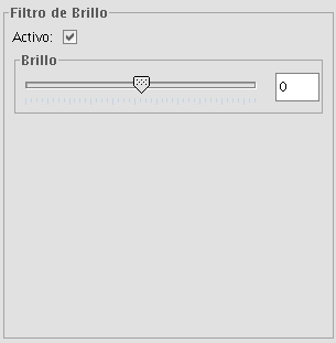
Brightness filter
The contrast filter changes the contrast value of the layer. You can increase or decrease the contrast by moving the position of the sliding bar or by entering the value directly in the text box and press enter.
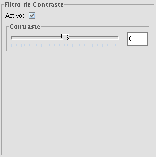
Contrast filter
Funciones espaciales
With this type of filter, graphical transformations like smoothing, edge detection, sharpening etc. are applied to the image.
The following filter types can be applied:
MEDIAN FILTER
The median filter applies a kernel of a certain size, which is determined by the user through the sliding bar labeled Window side.
The median filter is normally used to smoothen and to reduce noise in an image, by moving a kernel of N x N number of pixels over the image and evaluating each central pixel, replacing its value with the median of its neighboring pixels. Compared to the Mean filter, the advantage of the Median filter is that the final pixel value is a value that actually occurs in the image and not an average.
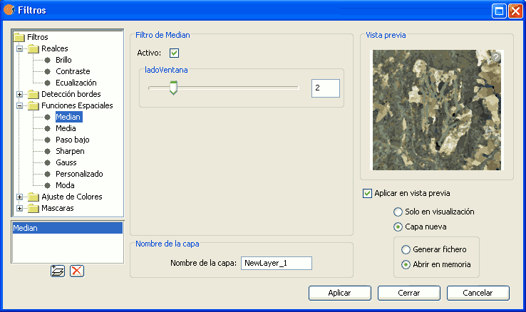
Median filter
MEAN FILTER
The mean filter applies a kernel of a certain size, which is determined by the user through the sliding bar labeled Window side.
The filter replaces the value of the central pixel with the mean value of the surrounding pixels. Each value of the kernel would be one and the divider would be the total number of elements in the kernel (i.e. a kernel of 3 x 3 would replace the value of the central pixel by the average value of the nine pixels covered by the kernel).
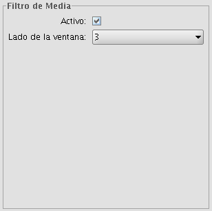
Mean filter
LOW PASS FILTER (smoothing filter)
The low pass filter applies a kernel of a certain size, which is determined by the user through the sliding bar labeled Window side.
Using a low pass filter tends to retain the low frequency information within an image while reducing the high frequency information.
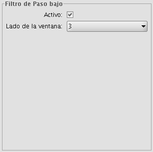
Low pass filter
SHARPENING FILTER
By moving the slider to change the sharpness (values from 1-100), the contrast of an image can be changed. The results can be evaluated in the preview window. With a higher contrast, details in the image can be accentuated but the noise will also increase.
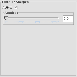
Sharpening filter
GAUSS FILTER
The Gauss filter applies a kernel of a certain size, which is determined by the user through the sliding bar labeled Window side.
The maximum value appears in the central pixel and gradually decreases for pixels that are further away from the central pixel.
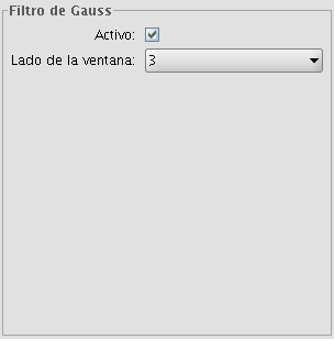
Gauss filter
CUSTOM FILTER
This is a kernel of 5 x 5 or 3 x 3, for which the values can be introduced by the user. After multiplying the pixel values with the kernel values, the result will be divided by the number specified in the Divisor textbox.
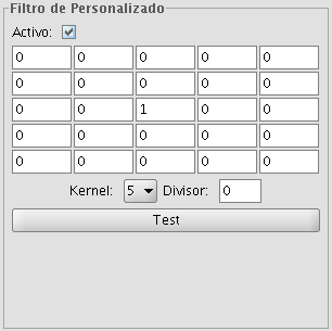
Custom filter
MODE FILTER
The mode filter applies a kernel of a certain size, which is determined by the user through the sliding bar labeled Window side.
This filter takes the value that occurs most in the surrounding pixels and assigns it to the central pixel.
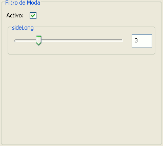
Moda filter
Ajuste de colores
Adjustment of RGB values
It is possible to change the balance between Red, Green and Blue in an image if needed. To do this, move the sliding bar to increase or decrease the values or enter the value directly in the text box next to the sliding bar. Ticking the "Brightness" check box ensures that the brightness level of the pixels will be maintained while the RGB values are changed.
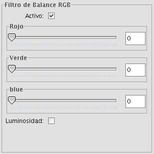
RGB balance filter
Adjustment of CMY values
It is possible to change the balance of Cyan, Magenta and Yellow in an image if needed. To do this, move the sliding bar to increase or decrease the values or enter the value directly in the text box next to the sliding bar. Ticking the "Brightness" check box ensures that the brightness level of the pixels will be maintained while the CMY values are changed.
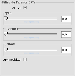
CMY balance filter
Adjustment of HBS values
It is possible to change the balance of Hue, Brightness and Saturation in an image if needed. To do this, move the sliding bar to increase or decrease the values or enter the value directly in the text box next to the sliding bar.
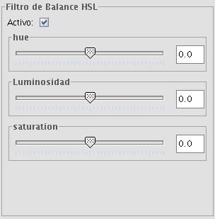
HBS balance filter
Detección de bordes
These filters attempt, through the use of kernels, to detect edges in the image and change the image so that these edges are enhanced, while the rest of the image is grayed out.
Filter dialog. Edge detection
There are four edge detection filters, all with the same interface and options, in which the user chooses a threshold in the range 0-255, and the possibility compare the results by ticking the compare check box:
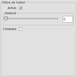
Sobel filter example
SOBEL
The Sobel filter detects the horizontal and vertical edges separately on a grayscale image. Colour images are converted to RGB gradations. The result is a transparent image with black lines and some remains of colour.
ROBERTS
The Roberts filter is suitable for detecting diagonal edges. It offers good performance in terms of location. The major drawback of this filter is its extreme sensitivity to noise and therefore has poor detection qualities.
PREWITT
The Prewit filter detects edges in all directions as it consists of 8 kernels that are applied over the image pixel by pixel.
FREI-CHEN
The Frei-Chen filter processes the neighbouring pixels as a function of their distance from the pixel that is being evaluated. The result is that edges in all directions are detected.
Máscaras
Transparent area
With this functionality it is possible to set the transparency level of a Region of Interest (ROI). The region of interest must have been defined previously. If the layer does not have a region of interest, the following message will appear: "A Region of Interest (ROI) must be defined for this layer to apply this filter. Please go to the dialog Area of Interest and select at least one ROI." If there are already one or more ROI associated with the layer, the message will not appear. Instead, a list of ROI will be shown, from which you can select one or more by ticking the corresponding check box. Then, adjust the level of transparency with the slide bar or by entering the value directly in the text box next to the slider. Ticking the check box labeled as "Inverse" will result in the opposite effect; all of the image except for the ROI will be set to the specified transparency level.
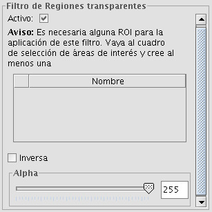
Transparent area filter
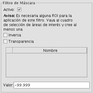
Mask
With this functionality it is possible to cut out a Region of Interest (ROI) that has been previously defined for the layer by assigning a fixed user-specified value to the rest of the image outside the ROI. If the layer does not have a region of interest, the following message will appear: "A Region of Interest (ROI) must be defined for this layer to apply this filter. Please go to the dialog Area of Interest and select at least one ROI." If there are already one or more ROI associated with the layer, the message will not appear. Instead, a list of ROI will be shown, from which you can select one or more by ticking the corresponding check box. Then, select the value to be assigned to the pixels outside the ROI by typing a number in the "value" text box. The default value is -99,999. Ticking the check box labeled as "Inverse" will result in the opposite effect; the ROI will be assigned the specified value while the rest of the image values are maintained.
Mask filter
Histograma
Descripción
To launch the histogram dialog window, use the drop-down toolbar selecting the "Raster Layer" button on the left and "Histogram" in the drop-down button on the right. Make sure that the text box that displays the current layer is set to the name of the raster layer for which you want to see the histogram.

Histogram icon
The Histogram dialog shows a histogram of the statistical distribution of pixel values in the current view. This information is often useful when you are trying to color balance an image. In the middle of the dialog you will see the graph on which you can right-click to show a context menu with general options for this kind of graphics.
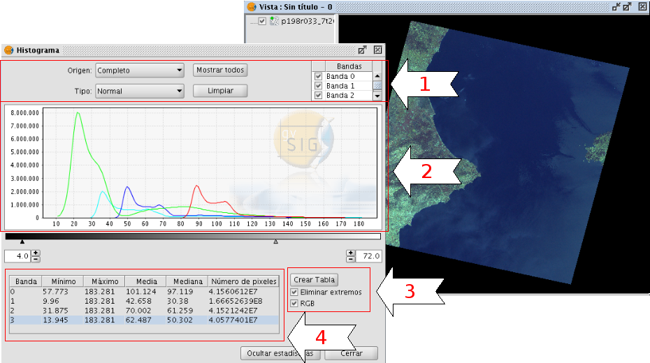
Histogram dialog window
In the upper part of the dialog (1) are the controls to configure the histogram:
1. Type of histogram
There are three types: "Normal", "Accumulated" and "Logarithmic".
- Normal: This is the normal histogram in which for every pixel value on the X axis the number of pixels is shown on the Y axis.
- Accumulated: Shows the accumulated number of pixels for every pixel value. The graph is therefore ascending.
- Logarithmic: Displays the histogram on a logarithmic Y axis, which may be useful for images that contain substantial areas of a constant value.
2. Data source
With this option you can select the data source for the histogram:
Current view (R,G,B):
With this option, the pixel values that are displayed in the current view of gvSIG will be used for the histogram. Therefore, the band selector shows only the R, G, and B values which are the visual bands. Every band will appear in its corresponding colour in the graph (red for R, green for G and blue for B). This is the default option when the histogram dialog is opened.
Complete histogram:
With this option, the histogram for the whole raster layer is calculated. Because of the amount of time that it would take to calculate the histogram for large images, the histogram is only calculated once and saved with a .rmf extension in the directory in which the image is stored. After the first time, the histogram for the same layer can be displayed much faster. (Keep in mind that if you delete the .rmf file that is stored with the image, you will lose its histogram information.)
3. Band selection
Apart from identifying to which band each histogram corresponds through its colour (in case of the current view Data Source) you can also identify the band by hovering the mouse over a point in the graph. The tooltip displays the band name and the value of the point.
Zoom operations
We can zoom in and out of the graph using the mouse.
- To zoom in on a part of the graph, draw a rectangle over it by pressing and dragging the mouse.
- To return to the original graph, click on the left mouse button on any point in the graph and drag to the left, then release the mouse button.
You can also zoom in and out using the context menu.
Context menu
When you right-click on any part of the graph, the context menu is shown with the following options:
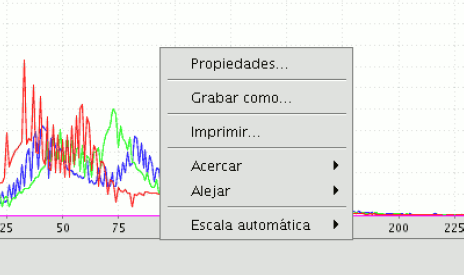
Histogram options. Context menu
- Properties: This will open the properties dialog of the graph, where you can configure characteristics such as the background colour, title, font etc.
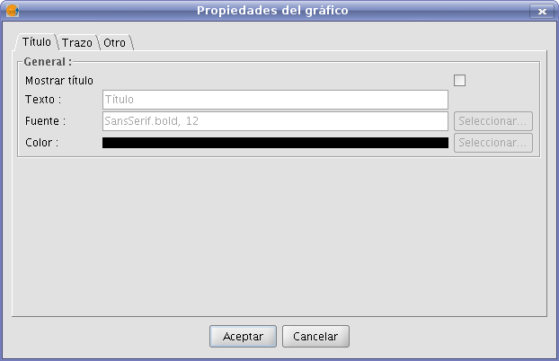
Histogram properties
- Save As: to save the graph as an image.
- Print: this opens the printer dialog from where you can print the graph.
- Zoom In: to zoom in on one or both of the axes.
- Zoom Out: to zoom out on one or both of the axes
- Auto Range: to adjust the zoom automatically to the window size, for one axis or for both.
5. Statistics (4)
The controls that appear under the graph allow the user to restrict the range of values (X axis of the histogram) on which the histogram is based. The default setting is the complete range so that, for example in a Byte data type image, the statistics are calculated for all the pixel values from 0 to 255. You can enter the values directly in the text boxes or use the + and – controls next to the text boxes. You can also slide the triangles over the sliding bar to select the range of values.

Sliding bar with pixel ranges
In this table, the statistics that correspond to the selected range of pixel values are shown in the text boxes. Each row of the table corresponds to one raster band as displayed in the histogram. The columns that are shown are:
- Minimum pixel value for the selected interval.
- Maximum pixel value for the selected interval.
- The mean (average) of all the pixel values for the selected interval in the histogram.
- Median pixel value for this interval.
- The number of pixels included in the selected interval.
6. Export the table (3)
You can export the table through the option "Save as DBF". The data contained in this table are the values of the current histogram. After creating the DBF table, it can be used as any other table in gvSIG.
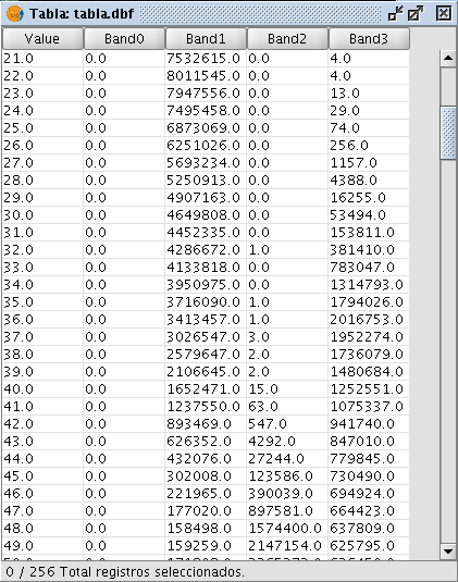
Resulting DBF table
Preferencias
The Raster section of the Preferences dialog contains the option "Number of classes" where you can set the number of intervals in which the histogram is divided when the data type of the image is not Byte. For Byte images, this value is 256. In the preferences dialog, the default value of this option is 64 but you can choose any of the options (32, 64, 128, and 256). The intervals are the parts in which the range of values is divided. For example, if we have a DTM with values between 0 and 1 and there are 64 intervals, each interval will have a range of 1/64.
The number of classes does not only refer to histograms but also to other functionalities that require a division in intervals of value ranges.
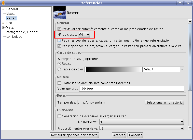
Raster Preferences
Información de la capa
Descripción
You can find information about the current raster layer through the option "Raster Properties", which shows a dialog with multiple tabs containing information about the raster layer. To get information about the layer, click the tab "Information".
The "Raster Properties" dialog can be accessed in two ways: by right-clicking on the raster layer in the Table of Contents or through the raster properties icon in the toolbar:

Raster Properties icon
Here, set the left button to Raster Layer and select the option Raster Properties from the pull-down button on the right. Make sure that the name of the raster layer for which you want to see information is displayed as current layer in the text box.
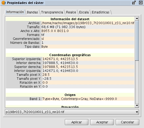
The Information tab of the Raster Properties window shows general information about the raster layer. Since a layer can consist of multiple files with the same geographic extension, you can choose the file for which you want to see information from the pull-down tool on the bottom of the "Information" tab window. The information is divided in thematic blocs with a header in bold letters indicating the bloc theme.
The bloc Dataset information shows the name of the file, disk size, width and height in pixels, data format (file extension), whether it is georeferenced, the number of bands and the data type.
The bloc Geographic coordinates shows the georeferencing information of the layer as well as the pixel size.
The bloc Origin will show an entry for each band in the file. For every band you can see the data type, the colour interpretation and the value that is assigned to NoData pixels. The colour interpretation of a band is important for the display on screen. If a band has an interpretation such as Red, this means that gvSIG will interpret this band to be displayed as the red band in RGB visualization. This colour interpretation will be used as default for the displaying of the image. A band may have the following types of representations: Red, Green, Blue, Gray, Undefined or Alpha. The NoData information associated with the band will not be taken into account when processing the image, and the NoData values can be shown as transparent if needed (see the section "NoData values").
The bloc Projection will show the projection information of the layer, if available. The representation format is WKT.
The bloc Metadata will show metadata information from the image header if available.
Raster Properties. Metadata
Rango de escalas
Descripción
To set the layer visibility according to scale range, you can specify the scale ranges in the "General" tab of the Raster Properties window.
The "Raster Properties" dialog can be accessed in two ways: by right-clicking on the raster layer in the Table of Contents, or through the Raster Properties icon in the toolbar:

Raster Properties icon
In the "General" tab, the scale ranges can be set as shown in the picture below:
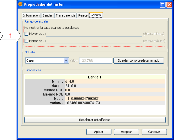
Raster Properties. Configure Scale ranges
There are two ways to hide the image according to its scale:
- Hide when the scale is bigger than 1:xxx, where xxx is a numeric value to be entered. This corresponds to the minimum scale.
- Hide when the scale is smaller than 1:xxx, where xxx is a numeric value to be entered. This corresponds to the maximum scale.
Realce (Propiedades)
Descripción
The Raster Properties dialog contains options for the enhancement of raster layers. The "Raster Properties" dialog can be accessed in two ways: by right-clicking on the raster layer in the Table of Contents or through the raster properties icon in the toolbar:

Raster Properties icon
Here, set the left button to Raster Layer and select the option Raster Properties from the pull-down button on the right. Make sure that the name of the raster layer for which you want to see information is displayed as current layer in the text box.
In the Raster Properties dialog, select the "Enhancement" tab.
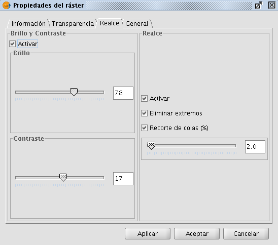
Raster Properties. Enhancement
Every modification in this Enhancement dialog will be applied to the current view for visual interpretation purposes and can not be saved as a new layer. If you want to save the enhancements, you will need to use the Filter dialog or the Radiometric Enhancement dialog, depending on whether you want to modify the brightness and contrast or apply a linear enhancement.
On the left side of the dialog, the controls for modifying brightness and contrast are shown. By default, these controls are disabled but if you want to change the values, you can activate them by ticking the "Activate" check box. Then, use the slide bar to alter the slide bar or type the value directly in the corresponding text box.
The right side of the dialog is used for linear enhancement. This is a simplification of linear radiometric enhancement to control the display of images of data types other than Byte. For Byte images, this control is disabled by default. For other data types, these values are automatically set when the raster layer is loaded. It is recommended to use this control only to modify automatically assigned values. For more enhancement options it is more appropriate to use the Radiometric Enhancement function.
The enhancement stretches the data over a range from 0 to 255 to improve visual interpretation. The option "Remove edges" will ignore the minimum and maximum values that appear in the image. The option "Clipping tail (%)" will sort the values from low to high, and cut off the values that are lower or higher than a specified percentage of the total number of values. The effect is a shift in the maximum and minimum values.
Salvar a raster
Descripción
The tool for exporting the view as an image can be accessed from the drop-down toolbar by selecting "Export to raster" on the left button and "Save view to georeferenced raster" on the right button. Make sure that the name of the raster layer that you want to export is set as the current layer in the text box.

Export to raster. Save view to georeferenced raster
A message will appear to inform that you can use the selection tool to set the area in the view to export.
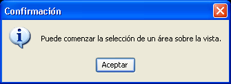
You can begin to select a area on the view
Now, you can select two points in the view to define the rectangle of the area to be exported, by clicking the first point and dragging the mouse towards the second point, then release.
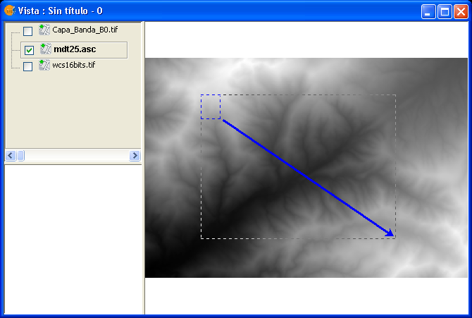
Selection of a rectangle to define the output image
Then, the Save view to georeferenced raster dialog will appear. If the selected area is too small, the dialog will not appear and a bigger rectangle must be selected.
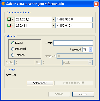
Save view to georeferenced raster dialog
The upper part of the Save view to georeferenced raster dialog shows the coordinates of the two points that define the selected area in the view. You can edit the coordinates to change the selected area.
In the option box in the central part of the dialog you can choose from three selection methods:
- Scale. Selecting this option will enable the Scale textbox and the pull-down box "Spatial resolution" which refers to the resolution in points per pixel (ppp) of the exported image. When entering a value in the Scale textbox and clicking enter, the values "Mts/pixel" and the size (Width and Height) will be recalculated for the output image.
- Mts/pixel (Meters per pixel): When selecting this option, the "Mts/Pixel" textbox is enabled. When you enter a value in the Mts/Pixel textbox and press enter, the values for "Scale" and size ("Width" and "Height") will be recalculated automatically for the output image.
- Size: When selecting this option, the text boxes to enter the "Width" and "Height" will be enabled. When you enter one of these values, the other will be calculated automatically to preserve the right proportions of the image. The other data ("Mtx/Pixel" and "Scale") will also be recalculated automatically. By default, the Width and Height values are displayed in Pixels, but you can select the units (Pixels, Cms, Mms, Mts, or Inches) in which you want to see these values.
NOTE: To save time and memory the maximum size of output images is limited to 20000 x 20000 pixels. If the intended output image is larger and you click on "Apply", gvSIG will display a message that the parameters must be changed before trying again.
Clicking the "Selection" button will open a file browser dialog where you can specify the output file. Depending on the type of file, the corresponding driver will be loaded (you will notice that the button on the right of the "Selection" button will change). For example, an output file .jp2 will open the properties dialog for Jpeg2000. The formats in which you can save are .TIF, .IMG, .BMP, .PGM, .PPM, .MPL, .RST, .JP2, .JPG, and .PNG. Furthermore but only on Linux kernel 2.4 you can also select ECW.
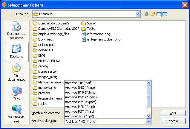
File browser dialog to save the output image
When you select the output file, the Properties button will be enabled.
For example, for geoTiff the dialog will look like this:
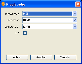
Properties geoTiff
- Photometric: [MINISBLACK | MINISWHITE | RGB | CMYK | YCBCR | CIELAB | ICCLAB | ITULAB]. This assigns the photometric interpretation. The default is RGB, as the input image consists of 3 bands of the Byte data type.
- Interleave: [BAND | PIXEL]. By default, tiff files are interleaved by band. Some applications only support interleaved by pixel, in which case you can change this option.
- Compression: [LZW | PACKBITS | DEFLATE | NONE] This refers to the data compression. The default option is NONE.
When the output image is selected and the properties set, you can click on "Apply". A progress bar will appear. Depending on the size of the output file, this process may take while. Processing times may vary between a few seconds or several days, so it is important to check the size of the output image in pixels before clicking "Apply". When finished, a screen with statistics will appear that indicates the path of the output image, the disk size, the duration of the process and whether it was compressed. To check the georeferencing of the output image, you can add it to the view as a new layer with transparency.
Realces Radiométricos
Descripción
The maps that are obtained through digital processing of satellite imagery are useful not only for thematic mapping, but also as a backdrop on which map features can be overlaid. If the visible bands are displayed in a colour composition through the colouring of each band with the corresponding colour gun, it is important that the bands are sufficiently enhanced so that the colours appear more natural. The final display colour depends not only on the direct result of the chosen colour composition but also on the radiometric post-processing. The satellite image map will be more useful as backdrop if the bands are enhanced and displayed in colours that match the natural colours as the human eye perceives them. gvSIG provides the enhancement tools to adjust the colours for each band.
In the following sections the different parts of the dialog are described:
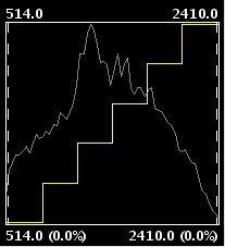
Histograms
The central part shows two graphs (1). The graph on the left is the histogram of the input image. The graph on the right shows the histogram of the output image. The graphs that are presented with a yellow line can be modified with the mouse. When you change the input histogram, the output histogram will be changed accordingly and you can preview the result.
In the upper corners of the input histogram are the maximum and minimum values of the raster displayed. In the lower corners, the maximum and minimum values that are being included in the enhancement are displayed. The percentage of values that are being left out of the histogram appears in parentheses. These values can be modified by grabbing and dragging the dotted vertical lines on the side of the graph. Dragging the left line will modify the minimum value, while dragging the right line will modify the maximum value. (This way, by leaving out the values that are not used in the input image, you can stretch the output values over the whole range of available values, so that the visual quality is improved.)
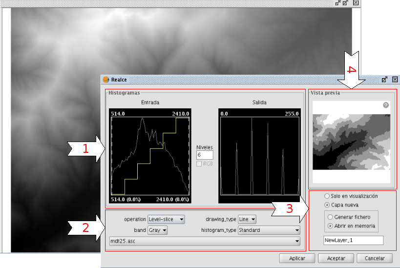
Radiometric Enhancement dialog
Controls
In the lower part of the dialog (2) you will find some controls with the following options:
Type of function:
The enhancements will replace each input value with an output value. This process is done by creating a look-up table which provides the correspondence between a range of input data and a range of output data. To apply this correspondence, a fuction is used. The used function and its parameters are chosen by the user.
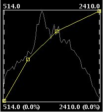
Linear enhancement
- Linear: Linear enhancements apply the correspondence between the input data and output data in a linear way. In the simplest case, a straight line will correlate each value in the input interval with the corresponding value in the output interval in a complete equidistant way. For example, if you have an output range between 0 and 255 and the input values are between 0 and 1, the input value 0.5 would result in an output value of 127.5. This is the default algorithm when you first open the radiometric enhancement dialog. Variations of this algorithm can be achieved by introducing break points in the yellow line, by clicking on the line at the point where you want to break it. You can remove break points by right-clicking on them. Existing break points can be moved by dragging them. The effect is that the linear filter is divided in parts with different inclination, so that different parts will follow a different linear function as defined by the inclination of the corresponding line part.
Linear radiometric enhancement
- Level slice (piecewise linear): This is a type of linear enhancement. It divides the function stepwise in equidistant parts. The effect is that the input values between two points on the same horizontal level will be assigned the same output values, so that the resulting image will have colour intervals without transitions. (This may be useful to highlight a specific range of gray levels in an image, for example to enhance certain features.) You can modify the number of intervals by changing the value in the text box labeled "Levels". The default value is 6 levels.
Piecewise linear enhancement
Non-linear enhancement
The non-linear enhancements have the same approach as the linear enhancements in the sense that each input value is replaced by an output value. The difference lays in the function that is assigned to produce the output values, which is non-linear. The available non-linear functions are logarithmic, exponential and square root. With each function you can modify the curve to smooth or accentuate the enhancement result.
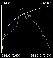
Exponential radiometric enhancement
Band
With this option you can specify the raster band to which the enhancements are applied. For a correct balance of the image, it is recommended to enhance each band separately.
Drawing type
With the option drawing type, different types of histograms can be chosen. Filled will draw a filled histogram while Line will only show the contours of the histogram. The colour of the line or fill pattern depends on the selected band. The bands Red, Green, Blue and Gray are displayed in red, green, blue and gray respectively.
Type of histogram
- Standard: Standard display of the histogram. For each possible value on the X axis, the number of pixels that are assigned this value in the output image are shown on the Y axis.
- Cumulative: For each possible pixel value on the X axis, the number of pixels that are assigned this value in the output image are shown on the Y axis. Furthermore, the number of pixels with the same or lower value are added to the result.
- Logarithmic: This shows the logarithmic value of the histogram in each position, resulting in a more balanced histogram without dominating peak values.
- Cumulative Logarithmic: This shows a cumulative histogram in logarithmic values.
RGB Check box
When check box labelled as RGB is ticked, it is assumed that the image is displayed as RGB with Byte data type and values between 0 and 255. If the checkbox is not ticked, it is assumed that the range of values are Byte data type values between -127 and 128, which will produce significant differences in the display and in the minimum and maximum values that are shown in the bottom of the input graph.
Display enhancement results
In the lower right part of the dialog (3), you can indicate how you want to see the enhancement results; in the current view or saved as a new layer.
Preview
The preview window (4) shows the real-time results of each enhancement that is applied to the image.
Salvar Como
Descripción
Raster layers can be exported to other raster formats through the Save As dialog. You can access this dialog from the drop-down toolbar, selecting the option "Export to Raster" on the left button and "Save As" on the drop-down button on the right. Make sure that the name of the raster layer that you want to export is set as the current layer in the text box.

Export to Raster - Save as
When selecting the option Save As, a file browser window will open where you can select the output file. On the right side of this dialog there is usually a control panel with various saving options. This control panel will look different depending on the driver for the selected output format, because every format has specific options. For some output formats there are no controls.
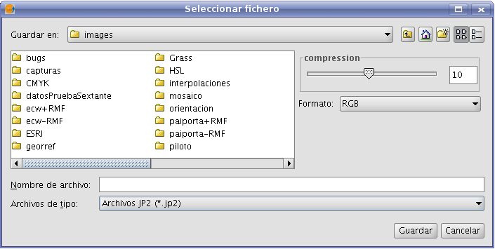
File selection dialog for Save As tool
Some of the most common options for the different formats are:
- Sliding bar labeled as "Compression" or "Quality": for formats with compression. The sliding bar is used to specify the extent to which the output image is to be compressed. The compression will affect the quality of the output image.
- Tfw: When this checkbox is ticked, a text file with georeferencing information will be generated. Depending on the input format, the extension of the georeferencing text file will be .tfw, jpgw or .wld.
- Interleave: the band interleaving of the output image; by pixel or by band. Some applications may require interleaving by pixel, and others interleaving by band to display the output image correctly.
- Compression: for formats such as .TIF there are several compression methods to choose from (LZW, Packbits, or Deflate)
- Photometric: photometric interpretation (RGB, CMY, ...) to be assigned to the result.
(Export raster formats are .TIF, .IMG, .BMP, .PGM, .PPM, .MPL, .RST, .JP2, .JPG, and .PNG)
Recorte de capas
Descripción
(The clipping tool can be accessed from the raster toolbar by selecting "export to raster" from the left drop-down button and "Clipping" from the drop-down button on the right. Make sure that the raster layer that you want to clip is set as the current layer in the text box.)
With the clipping tool, you can create new layers from an existing one. The options are:
- Extract an area from the input image to be saved as a new layer (cropping)
- Modify the resolution through various interpolation methods
- Modify the order or the number of bands
- Separate the bands into multiple files
Selection of the clipping area
In the "Coordinates" tab of the clipping dialog, there are text boxes to enter coordinates. In the upper part are the values in pixel coordinates and in the lower part the real coordinates. For each item, the two upper text boxes correspond to the coordinates of the upper left corner, while the lower two text boxes correspond to the lower right corner. When changing the pixel coordinates, the real coordinates are re-calculated automatically and vice versa.
There are 3 selection methods that will fill the coordinates automatically. These methods can be activated by clicking the buttons on the bottom of the clipping dialog. From right to left, the buttons are:
- "Select from the view". This is the most commonly used tool to clip a layer. After clicking this button you can draw a rectangle over the view to select the portion of the input layer to be saved as a new layer.
- "Full Extent of the raster layer" When clicking this button, the coordinates of the upper left and lower right corner of the input image are filled in the text boxes.
- "Fit to the maximum extent of the ROIs of the layer". When clicking this button, the extent of the area covered by the ROIs associated with the layer is calculated, and the coordinates are filled in the text boxes.
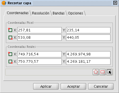
Clipping dialog. Coordinates tab
Modifying the resolution
In the "Spatial resolution" tab of the Clipping dialog, you can modify the resolution of an output image through various interpolation methods. There are two option boxes located on the upper part of this tab:
- Cell size: Ticking this option will activate the text box labeled "Cell", where you can introduce the new cell size value. By default, the text box shows the cell size of the input image.
- Width x Height: Ticking this option will activate the text boxes labeled "Width" and "Height" where you can introduce the desired width and height of the output image. When changing the width, the height will be re-calculated automatically and vice versa to maintain the correct proportions of the selected area.
When modifying the resolution it is necessary to resample and re-assign the pixel values for the output image through an interpolation method. There are four interpolation methods available: Nearest neighbour, Bilinear, inverse distance and B-Spline. The nearest neighbor is the fastest interpolation method, but the results in pixilation of the image and a lower visual quality. The other interpolation methods produce a smoother result.
The button labeled "Restore" returns the initial values of the input image.
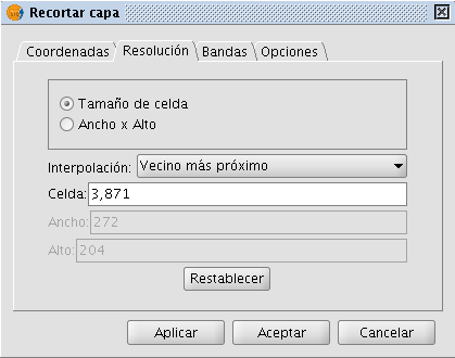
Clipping dialog. Spatial resolution tab
Band selection
The "Bands selection" tab of the Clipping dialog displays a table that lists the bands of the input image. When processed, the output image will have the bands in the order as shown in this list. By default, the output image will have the same order of bands as the input image. The order of the bands can be modified through the "Up" and "Down" buttons. The selected row will go up or down one position in the list. The bands can also be omitted from the resulting image by un-checking the corresponding row.
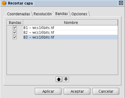
Clipping dialog. Bands selection tab
Selecting Options
The "Options" tab of the Clipping dialog presents various options that can be set by the user:
- Name of the output layer: you can modify the default name in the textbox labeled "Layer names". This is the name that will appear in the TOC and the name of the file that will be saved to disk. In case of several output layers (i.e. when each band is saved as a separate layer), the name will be the same for each layer but with a number at the end (_XXX). For example, if the layer is called NewLayer and there are 3 output layers, the respective layer names will be NewLayer_1.tif, NewLayer_2.tif and NewLayer_3.tif.
- If the check box labeled as "Create a layer for each band" is ticked, a new layer will be created for each band in the input image.
- If the check box labeled as "Save on disk automatically" is ticked, a text box labeled "Directory" will be activated where you can indicate the file path for the output files. If un-checked, the generated output layers are temporary.
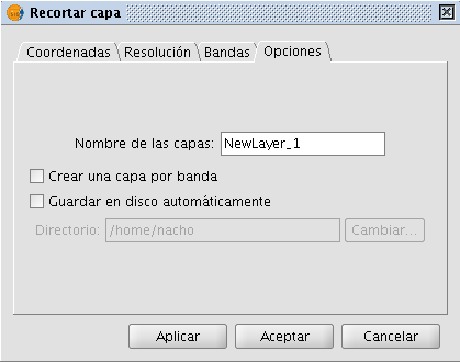
Clipping dialog. Options tab
Reproyección
Descripción
For the reprojection of raster layers, gvSIG uses the GDAL library. The reprojection process can be launched in two different ways: By activating the reprojection icon from the raster toolbar for images that have already been loaded to the view, or by reprojecting the layer before it is loaded to the view if this is needed.
The GDAL library does not support ecw, mrsid or jpeg2000 images and therefore images in these formats cannot be reprojected.
To launch the reprojection dialog from the raster toolbar, select "Geographic transformations" on the left drop-down button and "Reproject layer" on the drop-down button on the right. Make sure that the layer that you want to reproject is set as the current layer in the text box.

Image reprojection icon on the raster toolbar
When launching the reprojection function from the raster toolbar, a dialog opens which shows the projection information of the input image as "source projection". The source projection cannot be changed as it is assumed that the input layer has been loaded into the view with the correct projection. Under "target projection" the projection of the output image can be set by the user through the standard gvSIG dialog for CRS and transformations. It should be noted that not all transformations are supported; the projection options depend on the GDAL reprojection library.
The output layer can be saved on disk or opened in memory as temporary file. When the first option (which is the default) is selected, the user is prompted for a file name and path. Then, the reprojection process starts and when this is finished, it will ask whether you want to add the new layer to the TOC.

Reprojection dialog
NB: When reprojecting an image, the used transformation is "EPSG Transformation"; with raster layers the other transformations (manual, composed or grid) can not be used.
Images can also be reprojected before loading them to the view. To do this, you will need to have the option "Ask for projection when the raster loaded has different projection from view", located in the raster options section of the Preferences dialog, selected. If this option is selected and a raster with a different projection than the view is loaded, a dialog is opened with projection options. The default option is to load the layer while ignoring the projection, but you can reproject the layer by selecting the option "Reproject raster to the view projection". Then, the same Reprojection dialog is shown, but in this case the "target projection" is fixed to the projection of the view, and the "source projection" can be changed, as in some cases the projection of an image may not have been set correctly or the needed projection information maybe missing.
After accepting the settings, the reprojection process will start and the layer will be added to the TOC.

Reprojection options when loading an image to the view
Seleccionar Capas Raster
Descripción
Raster layers can be selected through the raster toolbar by selecting the option "Raster layer" on the left drop-down button and "Select raster layers" on the drop-down button on the right.

Select raster layer icon
When multiple raster layers have been loaded into the view, you can select one of those as current layer. By clicking on one of the layers in the TOC, the layer will be selected and its name will appear as current layer in the drop-down text box of the toolbar.
Tablas de color y gradientes
Descripción
The Colour table interface allows users to assign specific RGB values to a range of pixel values in a single band image. It is important to note that the input image can only have one band because if there are multiple bands, each of the bands will have colours associated with it. With the colour table functionality, users can build new tables or gradients, or modify existing ones.
The colour table dialog can be launched from the toolbar by selecting the option "Raster layer" on the left drop-down button and "Colour table" on the drop-down button on the right. Make sure that the name of the layer for which you want to build colour tables is set as the current layer in the text box. The "Colour table" option will only be available if a single band image is selected.

Colour table icon
To use this function, it is important to know the minimum and maximum values in the image. If these values are unknown, they will have to be calculated. Depending on the size of the image, this calculation process may take some time. When the Colour table dialog is launched for an image that does not have any colour tables associated with it, all components will be inactive. To get started, we need to tick the check box labelled "Activate color table".
Description of components
The colour table dialog is divided into several parts:
- The central part, which covers most of the dialog, displays the legend associated with the image in tabular or gradient form. (You can switch between table and gradient view by clicking on the tabs.)
- In the lower part are the controls with settings for the tabular and gradient view.
- A preview window is located in the upper right corner of the dialog. Here we can preview the output results before they are applied to the image.
- The library in the lower right corner lists the predefined colour tables. From this list, you can choose a colour table to apply to the image. It is also possible to create a new colour table and add it to the library for future use.
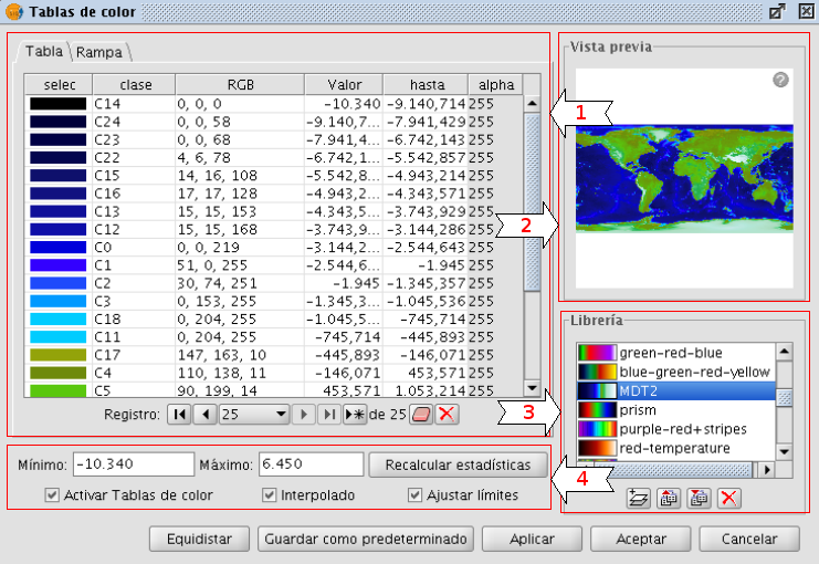
Colour table dialog - Table tab
Tabular view
Every row in the table corresponds to a range of pixel values and its associated RGB colour. The column Value shows the first value of the range and the column To shows the last value of the range. These values can be edited directly by double-clicking on the cell and typing a new value. The RGB column contains the RGB value to be assigned to the range of pixel values. The cells in this column are not editable, but if you want to change the colour you can go to the corresponding cell in the Colour column and click on it. A generic java colour selection dialog will appear where you can modify the colour by changing the RGB values or visually.
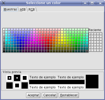
Colour selection
The Class column contains associated labels that will not have any effect on the calculation and are just meant to add descriptive names to the range of values. If there is any text in this column, it will be displayed in the map legend when this is created. The last column labelled Alpha shows transparency values. When clicking on the values, a transparency selection dialog will open.
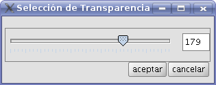
Apply transparency
To manage the rows of the table (add, delete or move) you can use the general table controls located below the table (see the table control description).
Gradient view
The gradient view (which can be accessed by clicking the gradient tab) contains the same information as the tabular view but presented in a different way, and with the possibility to obtain results that are difficult to achieve with the tabular view. The colour bar represents the range of values from minimum on the left to maximum on the right. At the start, the end and on intermediate points on the colour bar are a number of break points with a fixed colour value.

Break point
These break points indicate the colour that will be assigned to the value that falls on that point. A click on a break point will activate the text boxes below the colour bar. These text boxes show the following information about the selected break point:
- Colour: The colour of the break point (which can be modified by clicking on it)
- Class: Label associated with the point. This is the same associated label as in the Class column of the tabular view.
- Value: Pixel value at this break point.
To add a break point, just click below the colour bar. After adding a break point you can modify its information. To remove a break point you can click on it and drag it away.
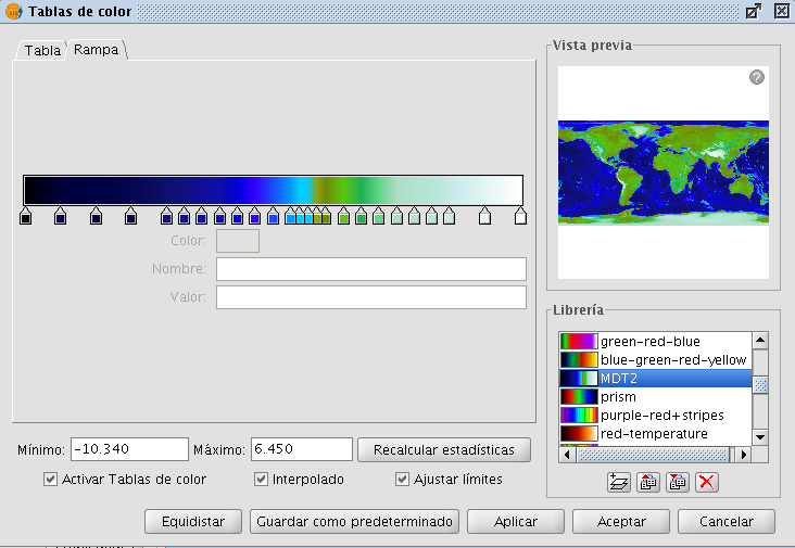
Colour table dialog - Gradient tab
The final result of the gradient will depend on whether the check box labelled as "Interpolated", located below the gradient tab, is ticked or not. This option is available both in the tabular view and the gradient view. When ticked, the transition between one break point colour and the next colour will be gradual. If it is not ticked, the transition will be abrupt. The point where one colour ends and the next colour begins is marked by a diamond-shaped symbol.

Cutoff point
This cutoff point can be moved to the right or the left by clicking and dragging it.
General controls
In the lower part of the dialog are the controls for the tabular and gradient view.
- The text boxes labelled "Minimum" and "Maximum" indicate the minimum and maximum values of the image. We can recalculate these values with the button labelled "Recalc Statistics".
- The check box labelled "Activate colour table" is used to enable or disable the use of colour tables for the current layer.
- Ticking the check box labelled as "Interpolated" will result in a smoother transition between the colours of two ranges of pixel values. This means that instead of assigning a fixed colour to the whole range of pixel values, the RGB colour value of the intermediate pixel values will be the result of an interpolation of the first colour in the range, the last colour in the range and the relative position of the pixel value. If you disable this check box, the transition between colours will be abrupt.
- The check box labelled "Limits adjust" is used to adjust the ranges to the maximum and minimum values of the image. If this is turned off, the colour table will be applied to the whole range of values which is 0 to 255 by default.
- Clicking the button "Middle distance" will result in break points that all hold the same distance between them (they will be equally spread over the colour bar). The first and last values of the range of pixel values will be modified accordingly in the tabular view.
- When clicking the button "Save as Default", the current colour table will be set as the default colour table for this image. The colour table information will be saved as a metadata file (.rmf) with the image, and the next time that the image is loaded in a gvSIG view it will have this colour table associated with it by default.
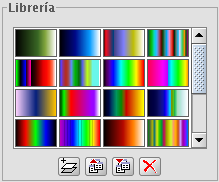
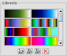
Library of colour tables
gvSIG provides a list of predefined colour tables to which you can add others that you have built yourself. Located at the lower right part of the Colour table dialog, the colour table libary allows users to scroll through and manage colour tables. The list of colour tables can be displayed in three ways: List, SmallIcon and LargeIcon. The type of display can be changed by right-clicking on the list, after which a drop-down menu appears where you can select the display mode.
List:
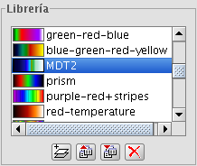
Colour table library - List display mode
SmallIcon:
Colour table library - SmallIcon display mode
LargeIcon:
Colour table library - LargeIcon display mode
Below the colour table library are buttons to add, export, import and delete colour tables
- When clicking on the button with the tooltip "New library", a dialog opens which prompts for basic information of the colour table: the name, minimum value, maximum value and the intervals. The default minimum and maximum values are 0 and 255. In principle there is no need to change these values because the colour table is automatically set to the value range of the image to which it is applied. The intervals can be specified by two different methods. The first method is by defining an interval of values, after which the number of intervals is calculated for the whole range of values. The second method is to specify the number of intervals, after which the size of the intervals is calculated automatically.
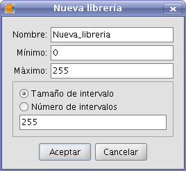
Create new colour table
- To remove colour tables press the button with the tooltip "Delete library". You will be prompted for confirmation before the selected colour table is deleted.
- You can export a colour table in one of the supported formats. Currently, only .rmf y .ggr y .gpl of Gimp are supported.
- You can import a colour table in one of the supported formats. Currently, only .rmf y .ggr y .gpl of Gimp are supported.
Legend in the view and map
The colour table built with this tool will classify the image in ranges of data values. When accepting the colour table dialog settings, this classification is shown in the TOC just below the layer name. For each colour, the corresponding range of values and the associated label, if any, is shown as a legend.
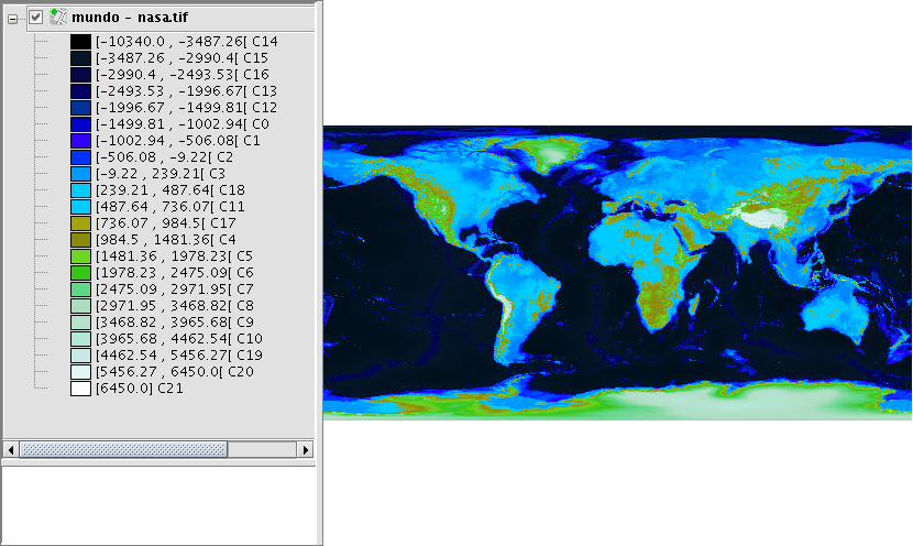
Legend in the ToC according to the colour table of the image
The generated legend can be inserted when preparing a map.
Map with view and legend inserted
Selector de bandas y ficheros
Descripción
You can find information about the current raster layer through the option "raster properties", which opens a dialog with several tabs. To access the list of image bands and corresponding files, go to the tab "Bands".
The "Raster Properties" dialog can be accessed in two ways: by right-clicking on the raster layer in the TOC, or through the raster toolbar by selecting "Raster layer" on the left drop-down button and "Raster properties" on the drop-down button on the right. Make sure that the name of the raster layer for which you want to see information is displayed as current layer in the text box.

Raster properties icon
The "Bands" tab of the "Raster properties" dialog provides options to select band combinations for image display. The upper part of the dialog shows a list of files of which the image consists. You can add more files, but they must correspond to the same geographic area. This is useful when you need to load several files of the same sensor, each file representing a band.
In the lower part of the dialog you can select the display order of the bands. By default, the display order is assigned by the colour interpretation of the bands, if that information is available. With the option buttons, you can change the display order by marking the bands that should be displayed in red (R), green (G), blue (B) or alpha (A). When clicking on the "Save" button, the colour interpretation information will be saved and set as default for the image. This means that the next time that the image is loaded in gvSIG, the display order of the bands will according to the settings that you have saved.
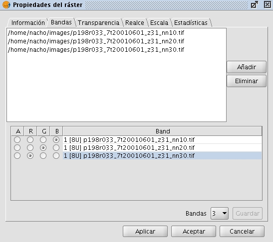
Raster properties. Band selection
Transparencia por pixel y opacidad
Descripción
You can find information about the current raster layer through the option "Raster properties", which opens a dialog with several tabs. To access the pixel transparency and opacity options, go to the tab "Transparency".
The "Raster Properties" dialog can be accessed in two ways: by right-clicking on the raster layer in the TOC, or through the raster toolbar by selecting "Raster layer" on the left drop-down button and "Raster properties" on the drop-down button on the right. Make sure that the name of the raster layer for which you want to see information is displayed as current layer in the text box.

Raster properties icon
The transparency options that are set here will only be applied to the current view (i.e. they will not be applied permanently to the image). The transparency will be calculated and applied each time when you zoom on the view. The transparency settings can be saved in the current project, and when the project is opened again, the transparency will be applied on the layer. However, if the same image is opened in another project, it will be displayed normally without the transparency settings.
The upper part of the "Transparency" tab of the "Raster properties" dialog shows a sliding bar labelled "Opacity". After activating the sliding bar by ticking the check box, you can modify the opacity of the whole layer by moving the slider. (Opacity is the opposite of transparency: if you set the opacity to 0%, the layer will be 100% transparent.)
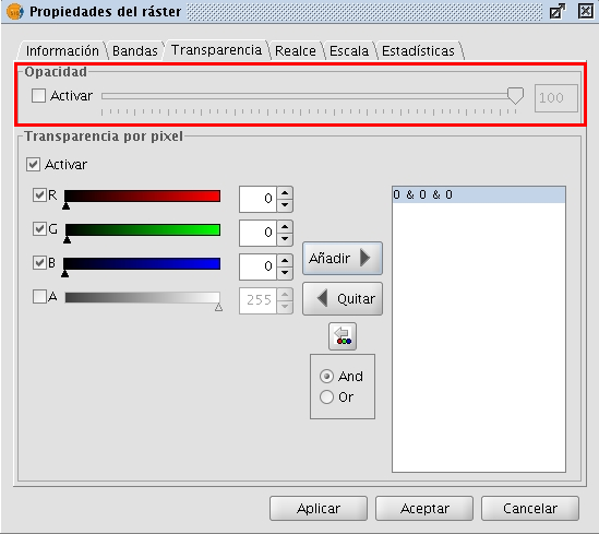
Set the transparency using the Opacity slider
The pixel transparency controls are located in the lower part of the "Transparency" tab. With these controls, you can apply transparency to pixels or a range of pixels depending on their RGB value. After activating the controls (by ticking the "Activate" check box) you can add specific RGB values to the list of elements through the "Add" button. Three values separated by the "&" or "|" symbol will be added as one item in the list; the three values correspond to the RGB value that will be set transparent. The values that are added are those that appear in the text boxes, the alpha value is optional. The information in these text boxes can be modified in three ways: typing the value directly by using the keyboard, moving the colour sliders on the left of the text boxes, or by clicking on the image in the view to select a specific colour value. This last option is activated with the button with the tooltip "Select RGB clicking on view". This will activate a crosshair cursor in the gvSIG view so that you can click on the image pixels and select the values for which you want to set the transparency.
If the line "255 & 0 & 0" is added to the list, this means that all pixels with the RGB values of 255 for red, 0 for green and 0 for blue (i.e. all pixels that are pure red) will be set transparent. The "&" symbol can be changed by the "And" and "Or" options. If "Or" is activated, the entries in the list will appear with the pipe symbol "|". The line "255 | 0 | 0" means that all pixels that have RGB values of 255 for red, or 0 for green, or 0 for blue will be set transparent. In this case many more pixels will be set transparent.
Set the transparency for specific pixel values
Valores NoData
Descripción
The NoData value refers to information that is not taken into account during the data processing. This NoData information is defined as one specific value depending on the data type of the raster layer. These NoData values can be set as transparent in gvSIG, because if these values do not represent relevant information, you may not want to display them. The value is associated with the raster layer (i.e. each image can have a different NoData value) and can be defined in the metadata or assigned by the user.
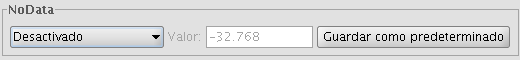
Raster properties. NoData value
To find out if the layer contains NoData values, you can open the "Raster properties" dialog and select the "General" tab where the NoData information is shown.
A layer can have an associated NoData value defined in its metadata. In this case, the text "Layer" is displayed in the drop-down text box in the NoData section. This means that the NoData value associated with the layer is being used. The text box labelled as "Value" shows the numeric value. In case the layer does not have a NoData value associated with it, the text "Deactivate" is shown in the drop-down text box while the "Value" text box is inactive and the value in this text box is irrelevant. If you want to define a new NoData value for the layer, either because the current NoData value is incorrect or because the NoData value is not defined, you can select the option "Custom". When selecting this option, the "Value" textbox will show the default NoData value as set in the "Preferences" dialog. You can modify this default value if needed.
By clicking "Apply" or "Accept" the new value is assigned to the layer. Keep in mind that the NoData values defined in this way are only temporary; when the layer is opened again this value will have been lost. To associate the new value with the layer you can click the button "Save as default", after which a message appears to confirm this action: "The default NoData value will be changed. Would you like to continue?"
Preferencias
The "Raster" section of the "Preferences" dialog contains options for "NoData" values. Here, you can specify whether you want to display the NoData values in the layers that are loaded into gvSIG.
The option "Set NoData value to transparent" does exactly what it announces; for any raster layer that is loaded into gvSIG and has associated NoData values (as defined in its metadata or assigned by the user), the NoData values will not be displayed. For efficiency in displaying images, this option is disabled by default.
Another available option is to change the default NoData value. When in the "Layer Properties" dialog the "Custom" option is selected, the NoData value that will appear is the default NoData value as set in this text box in the "Preferences" dialog.
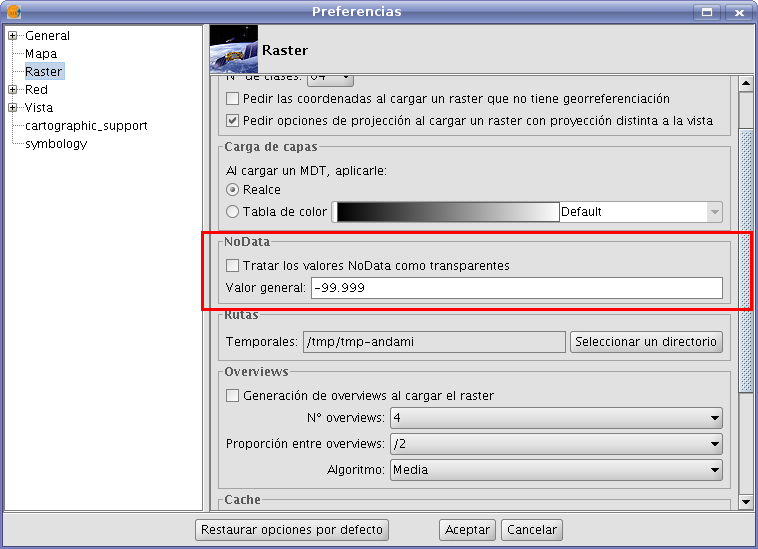
Raster preferences. Set default NoData value
Zoom a la resolución del raster
Descripción
You can zoom to raster resolution by right-clicking on the layer in the TOC. In the context menu that appears, click "Zoom to raster resolution".
This will activate a crosshair cursor in the gvSIG view which allows users to perform an action by clicking somewhere in the view. The action in this case is that with every mouse-click, the view will be centered on the point where you clicked. In addition, the view will zoom so that one screen pixel is the same size as a pixel in the current raster layer.
Vectorización automática
Descripción
The "automatic vectorization" function can be launched from the raster toolbar by selecting "Raster process" on the left drop-down button and "Vectorization" on the drop-down button on the right. Make sure that the name of the raster layer that you want to vectorize is displayed as current layer in the text box.

Vectorization icon
With automatic vectorization, you can generate a vector layer from a raster image using preprocessing to highlight the features of interest.
When launching the Vectorization dialog, the first step is to select the area of the image that you want to vectorize. Keep in mind that the vectorization process may take a long time, so it is recommended to minimize the area (number of pixels) for vectorization. The selection of the area for vectorization can be done in several ways. You can type the coordinates directly; either in pixel coordinates or in the map coordinates. The area can also be selected from the view by clicking the button "Select from the view", after which you can draw an approximate rectangle to define the area. Another selection option is by Region Of Interest (ROI). You can define a ROI here or use a previously defined ROI to set the area for vectorization. In the section "ROI selection" appears a list of available ROI and a checkbox next to each of these to select one or more ROI that you want to use. There are two options to vectorize the ROI: to vectorize the entire area inside the rectangle (bounding box) that covers all the selected ROI, or vectorize only the areas inside the ROI while considering the values outside the ROI as NoData values, excluding them from the calculations.
Finally you can select the scale of the image to preprocess. This is useful because a higher resolution of the preprocessed image will result in a higher precision for the resulting vector layer. You can define this with the drop-down text box labelled "Output Scale". By default, the resolution will be the same as the input image.
When moving on to the next step of the wizard, the process of cutting the image for preprocessing is started. A progress bar appears with the warning that this operation could take a few minutes. The resulting image cut is saved in the temporary folder of gvSIG.

Vectorization. Selection of the area to vectorize
There are two methods to preprocess a raster image to vectorize. The first is by creating a limited number of grayscale levels from the original image. The image will be converted to grayscale using one single band or a combination of bands (use the drop-down button labelled "Bands"). For the conversion to grayscale, a posterization process is used to reduce the number of different values. (By default, the image is reduced into 2 levels only: black and white.) For this process you can control the threshold on which the values are passing from black to white and vice versa. This can be done by moving the "Treshold" slider while you can see a preview of the result. (The Treshold slider is only available when there are 2 levels; when there are intermediate grayscale levels, the slider is disabled.) In addition to the posterization threshold, you can apply a mode filter or a noise filter to smoothen the result.

Vectorization. Conversion to grayscale
The second preprocessing method is useful to vectorize contour lines and can be applied to data types other than byte. With this method you can define intervals between each contour line to be vectorized. You can specify the number of intervals in which you want to divide the raster, or indicate the size of each interval. The cuts that have been selected will be shown on a graph that represents the histogram of the image. On this graph, you can modify the distance between cuts, or add or remove some of them using the mouse. It is also possible to modify the distance between cuts in numeric format using the table on the right of the histogram. Each entry in the table represents a cut with the corresponding value. This type of preprocessing is used for digital elevation models (for example .adf or .asc images).
When moving on to the last step of the vectorization wizard, the preprocessed image is generated with the specified values, and saved in the temporary directory of gvSIG.

Vectorization. Define intervals for vectorization in case of Digital Elevation Models
The last step is to select the method for generation of vectors. There are two methods: contour and potrace, that can be selected from the drop-down button after which a panel appears with settings that are specific for the method. The first method is the simplest and does not have any options. This method will trace the vectors in straight sections going through the pixel centers. This generates a network of vectors based on very small straight sections. The potrace method uses the potrace library for vectorization. The available options for this method are those that the potrace library provides and they are used to define the precision of the tracing of the curves: number of points for each curve, threshold, optimization, etc.

Vectorization. Options for vector generation
When clicking on "Apply" or "Accept", the process of vectorization will start after which you will be prompted whether to display the generated layer in the TOC.
Vista de análisis
Descripción
The "Analysis view" can be launched from the raster toolbar by selecting "Raster layer" from the left drop-down button and "Analysis View" on the drop-down button on the right. Make sure that the name of the raster layer that you want to analyze is displayed as current layer in the text box.

Analysis View icon
With this functionality you can zoom in on the current raster layer with 3 different zoom levels:
- On the left of the view, the layer is added to the locator map of gvSIG. This provides a general view of the layer, and you can zoom into the locator map by clicking and dragging, thus drawing a red rectangle. The area inside the red rectangle will be displayed in the view.
- The view itself is the second zoom level which functions independently, and the zoom variations that are performed on the view will be applied to the locator map as well so that it keeps being centered on the correct area.
- When launching the Analysis view, a small floating window labelled "Cursor Zoom" appears in the upper right corner of gvSIG. This window has the highest zoom level. The zoom level is fixed and always centered on the mouse point. By moving the mouse over the gvSIG view, you will see the contents change.
You can change the relation between the zoom level of this floating window and the gvSIG view. This is done by right-clicking on the floating window and selecting one of the values that are shown in the drop-down menu that appears. The available options are x4, x8, x16, and x32. This means that the pixels in the floating window will be 4, 8, 16, or 32 times bigger than the original.
The floating window also shows the RGB values of the pixel on which the cursor is currently located. The text colour of the RGB values as well as the colour of the central cross (red by default) can be changed by right-clicking on the floating window and choosing the option from the drop-down menu.
Keep in mind that, to see the effects in the floating window while moving the mouse over the view, the view must be active. If it is not active, just click on the view. When the cursor is outside the view, the content of the floating window appears black.
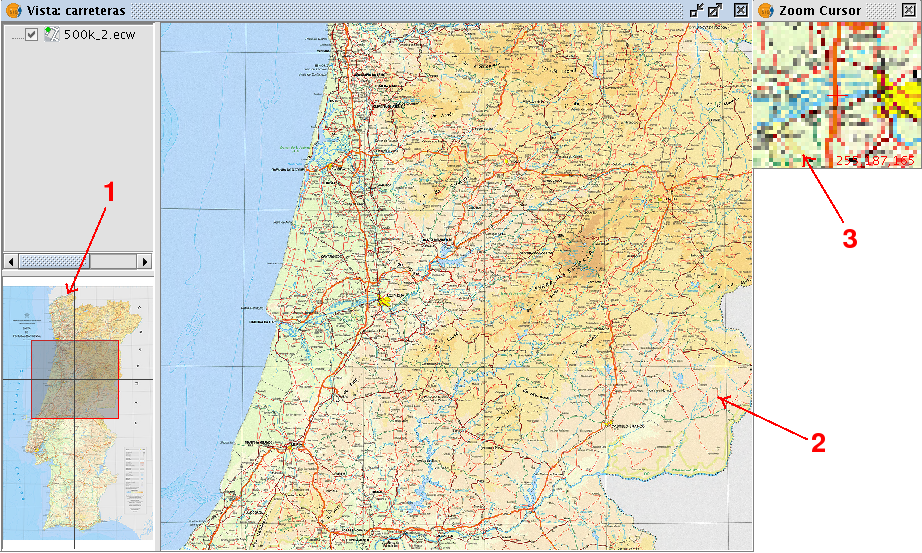
Screenshot with the different elements of Analysis View
There can only be one Analysis view open at any time in gvSIG. Therefore, the button "Analysis View" is re-labelled as "Close Analysis View" when the Analysis view is already open, so that it can be closed before re-opening.
Componentes generales
Vista previa
Descripción
A preview is usually shown for functions that require extensive processing. It is usually located in the upper right corner of the dialog as shown in the following example:
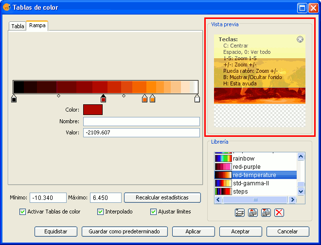
Component 'Preview'
The preview gives only an indication of how the final output will look like. Since only a minimum amount of data is used to generate the preview, the final result may be different.
The following options are available for preview windows:
- Move the image with the left mouse button.
- Center the image in the preview by pressing the C key.
- Zoom out to see the whole image with the space bar or 0
- Predefined zooms with keys 1 to 5. 1 gives a 1/1 zoom.
- Zoom with the mouse wheel or arrow keys + and -.
- Show a grid on the background to view images with transparency by pressing the B key.
- Access the help function by pressing the H key or clicking on the question mark in the upper right corner of the preview window.
The access to these preview functions through the shortcut keys only works when the focus is on the preview window, after clicking on it with the mouse.
For different types of functionality, the preview may appear with a different default zoom level. For example, the preview of colour tables is shown as completely zoomed out so that the effects on the whole image can be previewed.
Selector de resultados
Descripción
The output selection control is used to create new layers.
In this example the output selection control is shown in the lower right corner of the dialog (1):
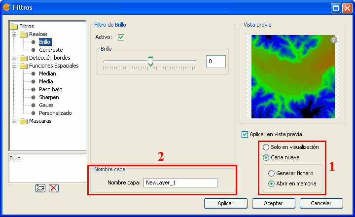
Output file selection
The selector consists of two components:
- For the output image, you can choose whether to apply the filters over the image in the current view (only for display) or save the output as a new layer.
- The option "Only on visualization" does not change the original layer, but will apply the list of filters when drawing and re-drawing the view. This option is faster when the image is very large (as the filters are only applied to the current view, not to the whole image), but it slows down the drawing and re-drawing of the view.
- The option "New Layer" will apply all the filters to the image and save the output to a new layer. This is faster when the image size is medium or small and the applied changes are considerable. The generation of the new layer will take some time, but then the displaying is as fast as it would be without the filters.
Both options have advantages and disadvantages, and it is up to the user to decide which option to choose.
- When selecting the option "New Layer", a second option control is enabled in which you can choose whether to save the layer to disk (Create file) with a file name specified in the text box (2), or to create a temporary gvSIG layer (Open in memory).
The new layer will be added to the view, and the TOC will show the layer name as specified in the text box.
** Note: The temporary working space of gvSIG is cleaned automatically, so any temporary layers will be deleted when exiting the application.
Control de tablas
Descripción
The table control component is used to represent data in tabular form and allows you to edit the data.
The possibilities are:
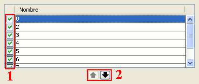
Table control components (1 and 2)
- Selection of rows in the table.
- Reordering the rows. Click on the arrow buttons to move a selected row up or down.
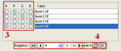
Table control components (3 and 4)
Choose a unique property for every row. In the example above, a band is allocated for each layer.
Typical table controls, as shown in the example at the bottom of the table. From left to right:
- Select the first row.
- Select the previous row.
- Drop down to select a particular row.
- Select the next row.
- Select the last row.
- Create a new row.
- Delete the selected row.
- Delete all rows from the table.
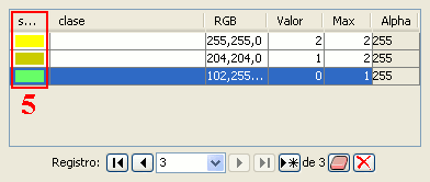
Table control components (5)
- In the table control, besides being able to edit anything if editing is enabled, you can also change the color by clicking on it.
Barra de progreso
Descripción
When running processes that may take a considerable amount of time, a progress bar is shown.
The progress bar indicates that a process is running in the background and informs the user on the status of the process at any given moment and on how much time has elapsed since the process started.
In the image below, you can see a screenshot of the progress bar during a running process.
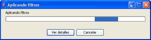
Progress bar component
The progress bar consists of several parts. The title indicates which process is running. Below the title, the current task that is being processed is indicated as well as the percentage of the process that has been completed.
The progress bar contains two buttons. To see more details, you can click the left button, after which the dialog is enlarged to display additional information as in the screenshot below.
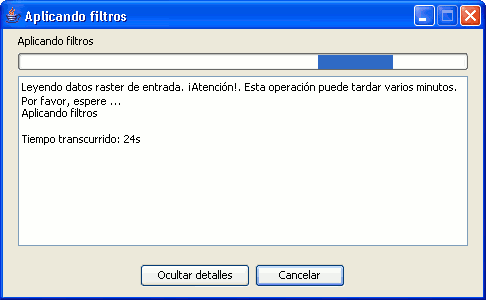
Progress bar with details
The additional information includes a list of tasks that have been performed and an indication of how much time has elapsed since the process was started.
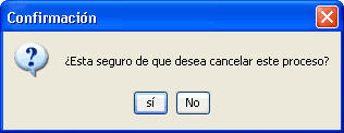
Confirmation message: are you sure you want to cancel this process?
If you want to cancel a process, you can click on the "Cancel" button on the right. A message will appear to prompt for confirmation. Clicking on the "Cancel" button does not always guarantee that the process is stopped immediately. Depending on the process, certain tasks might be needed to reverse the process and return to the previous state.
Estadísticas finales de generación de capa
Descripción
When processes that display a progress bar have ended, a statistics window with details of the process is usually shown.
Examples of such processes that launch statistics windows are Filters, Crop, Save As, etc.
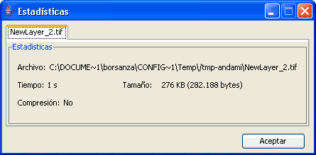
Statistics component
The statistics window shows the following information:
- File: Complete file path where the image has been stored.
- Time: The time that it took to complete the process.
- Size: File size on disk.
- Compression: Whether or not the image file has been compressed.
If you have generated more than one layer in the same process (as is the case when cropping images with multiple bands) the statistics window will display the information of each layer in a different tab.
The window can be closed by pressing the OK button.
Barra de herramientas desplegable
Descripción
With the increase of image processing functions in the menu of gvSIG, the toolbar had to incorporate these Raster functions by grouping them as pull-down buttons.
As can be seen in the image below, when a view is selected, a control will appear at the right side of the toolbar.
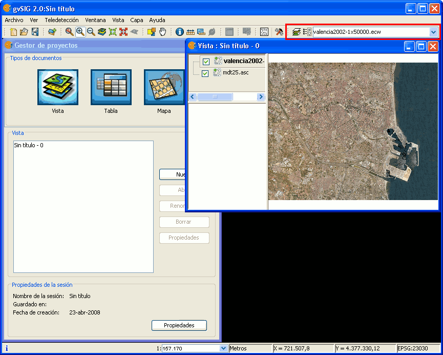
Drop-down buttons for raster functions in the toolbar
The control has two drop-down buttons and a search combobox with the name of the current layer.
The buttons work as follows (see image below):
Raster drop-down button, with two zones (1 and 2)
- Clicking in this area will change the visible order of the button.
- Clicking the area with the pointing down arrow shows the menu of options.
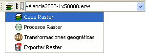
Groups of raster functions
With the first drop down button you can access a set of grouped functions. For each group of functions, the individual functions within that group will be shown in the second button. Therefore, the functions that are available in the second button depend on the group of functions that is chosen with the first button.
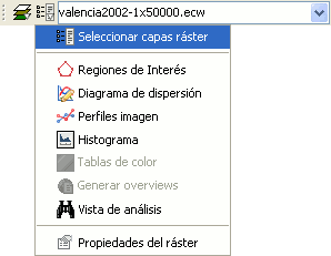
Individual raster functions shown in the second drop-down button
In the image above, the individual functions from the second drop-down are shown while in the first drop-down button the function group "Raster layer" is selected.
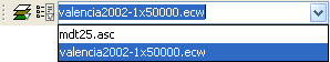
Combobox with the name of the current raster layer
The search combobox is used to select one of the layers in the TOC. When clicking on the arrow on the right, all the possible layers are shown.
Search Combo to select a raster layer
You can write text in the combobox to filter the list of images (i.e. write "1x5" to show only layers that have these characters in their name).
Transformaciones geográficas
Geolocalización
Descripción
The Geolocation tool provides the ability to change the related transformation that is applied to a raster in its display. A raster could have coordinates that place it in a geographical position. This geographic location is only a change of position, scale and rotation of the image relative to an original position. These changes in position, scale and rotation are those that can be changed with this tool. This can be done numerically and by visual approximation.
This tool does not provide capabilities to deal with complex projections and georeferencing involving the need for resampling.
To launch the geolocation dialogue of the layer, the drop-down toolbar is used by selecting "Geographical Transformations" on the left button and "Geolocation" on the dropdown button on the right. Make sure that the text shows the name of the layer to which we like to assign the transformation.

Geolocation Tool
Upon activating the geolocation tool on a raster layer, a small dialog will appear floating on the view with a series of text entries and a button bar. Also the raster layer that has been selected acquires the capacity to be moved, rotated or moved by clicking and dragging it to the right place on the view.
Transformation on the view
- Translation: When the geolocation tool is active you can move the mouse over the image on the screen and the cursor changes to a hand. This indicates that we can move by clicking and dragging on the raster view.
- Scaling: When the geolocation tool is active you can move the mouse over the edges of the image on screen and the mouse cursor will change. Depending on the chosen edge the cursor will take one form or another. If placed in the top or bottom borders the cursor will become a vertical arrow. This indicates that we can click and drag to scale the image from one side only. The scaling at all times keep the proportions of the raster. If we move the cursor around the side edges the pointer becomes a horizontal arrow now allowing us to scale laterally. In the case of the corners the cursor appears as an oblique arrow.
- Rotation: When the geolocation tool is active, we can move the mouse over the outer corners of the image and the cursor will change. This will appear as a circular arrow. This indicates that we can begin to rotate the raster from the selected corner.
- Shear: When the geolocation tool is active you can move your mouse over the outer side edges of the image and the mouse cursor will change. This will appear as an arrow with a symbol X or Y depending on whether the mouse is in the horizontal or vertical edges respectively. This indicates that we can begin to warp the raster in the direction of the X or the Y.
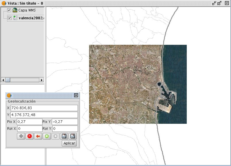
Vista Panel Image Geolocation
Transformation by introducing coordinates
From the geolocation floating box we can modify the transformation of the image on the view. The text entries marked as X, Y, Pix X, Pix Y, Rot X, Rot Y contain the current position in upper left X coordinate, upper left Y coordinate, pixel size in X, pixel size in Y, rotation in X and rotation in Y respectively. If we change these values from the keyboard these will be updated on the image by pressing the "Enter" key while the cursor is inside the text box or when it loses focus.
Controls of the geolocation box
Centering the raster layer in the view: With this button we center the raster in the current view regardless of zoom it has selected. The coordinates will be automatically calculated.
- Initialize the raster transformation: Resets all the transformations that have been applied to the cells back to the default.
- Go to the first processing: Assign the first transformation that was applied.
- Go to the previous transformation: Assign the previous transformation to the current that was applied.
- Go to the next transformation: Assigns the following to the current transformation.
- Upload georeferencing from tfw file: If we have a tfw file with georeferencing coordinates, these can be loaded with this option. A dialog to select the file you want will show up. The extension of the file must be tfw or wld.
- Save current transformation as the default for the raster: Applying this option saves the currently active transformation in the file .rmf attached to raster. Next time the raster is loaded will be with that transformation.
Modificar georreferenciación en la carga
Descripción
When you load a file that is not georeferenced, gvSIG can prompt you to enter the coordinates manually. For this the option has to be activated in preferences, which is disabled by default. The option that needs to be activated is "Pedir las coordenadas al cargar un raster que no tiene georreferenciación".
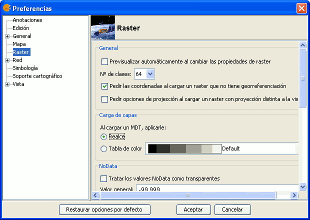
Raster Preferences. Pedir las coordenadas al cargar un raster que no tiene georreferenciación
In this case we will see a dialog with the message: "Name of layer. The layer has no georeferencing. Do you want to enter them manually?". If you answered "No", the load is carried out with the coordinates (0, 0) in the top left corner (width in pixels, height in pixels) in the lower right corner. If the answer is "Yes", then a dialog to enter the coordinates of the raster will show. In this one must be careful to enter valid data to avoid erroneous results. The dialog has two tabs from which we can enter the coordinates in the form of affine transformation or the upper-left and bottom-right corners. In the first mode will need the X and Y coordinates of the upper right corner of the original raster, the pixel size in X, the pixel size on Y, X rotation and the rotation Y.
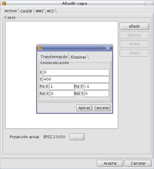
Loading raster without georeference. Transformation
In the second mode we only introduce the coordinates of the corners in the order indicated by the graphs.
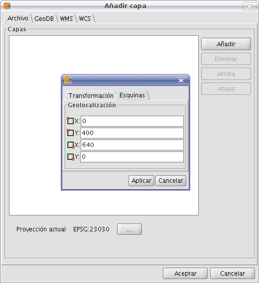
Loading raster without georeference. Corners
Georreferenciación
Descripción
Direct traslation from Google traslator
To launch the georeferencing dialog it is used the dropdown toolbar selecting the "Geographic Transformations" button on the left and "Georeferencing" from the dropdown button on the right.

Georeferencing Tool
Initially we must decide what type of georeferencing to implement, "reference maps" or "without reference maps".
Georeferencing with "Mapping Reference"
Start Dialogue georeferencing
To implement this type of georeferencing is imperative that we have previously charged in a view mapping that we will provide a geographic reference for taking control points. In case of not having it will close the options dialog georeferencing and proceed to prepare for the hearing. Once we have the view with reference maps georeferencing tool launched will see that the option "reference maps" is checked by default. Below is a dropdown menu which lists the views that gvSIG has at that time. If you have several it must select a view which is our base mapping for decision-points.
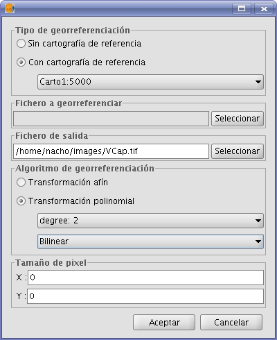
Dialog Georeferencing
In the panel marked "a georeferenced file" pops up a dialog for selecting the file for which you want to create checkpoints and later georeferencing.
The panel labeled "Output File" we must put the path and file name destination if the georeferencing is done with resampling. This option can vary from box options once we are inside the application, so it is not essential to a correct value at the moment, but if must be done before the end of the process.
The panel "georeferencing algorithm" select how we will get the output result. There are two possibilities, "affine transformation" and "polynomial transformation".
The affine transformation applied to raster an affine transformation only to the calculations performed with the control points taken. The affine transformation applied will be allocated "on the fly" for the display and the output image is the same as the input. The result of this transformation is therefore a georeferencing file. Keep in mind that this type of transformation is limited and the user will be responsible for selecting the most convenient transformation in each case.
The polynomial transformation involves a resampling of the input image taking into account the reference control points and obtaining an output image with deformations necessary to adapt to the new location. If you select this option we will be forced to decide the degree of transformation that we apply and the type of interpolation that we want to apply for calculating new pixels. Depending on whether you choose one degree or another need a minimum number of control points for them. This number of points required is given by the formula (order + 1) * (order + 2) / 2, ie for a polynomial of degree one will be needed at least three points, to grade two will need six points for third grade ten points ... The interpolation method affects the way we calculate the information that we have not. When an image georeferenced output image has deformations with respect to the original there are areas where no information is available. These can not be empty with what must be calculated from the areas where we know. These calculations can be performed by various methods, the simplest of these is "Nearest neighbor" which will be unknown pixel information closest known pixel. Other methods such as "bilinear" or "bicubic" make calculations using the known group of pixels surrounding the unknown. These other methods give a more relaxed but it is slower in its implementation. This option can vary from box options once we're inside the application.
The panel "Pixel Pitch" is the pixel size information of the output image. In principle this will be calculated from the input image but can be changed manually. This option can vary from box options once we are inside the application, so it is not essential to a correct value at this time.
The views
Executing the application are two views. The left contains the base mapping that we carry in the gvSIG view of the right and the image we want to georeference. Both have a control bar on the right for view actions. Also in the upper left corner are the coordinates of the mouse cursor. In reference mapping coordinates are those of the real world. In the image to be georeferenced coordinates in pixel coordinate on the upper left.
Cursor Zoom
In the central part appears a cursor with a central window. The window cursor is active when the view can be resized and moved. The contents of this window will be on display in the zoom windows. Ca da vista has its associated zoom window at the bottom. Par resize window cursor select the view you want by clicking on it then bring the mouse to the edges of the window until the pointer changes to horizontal or vertical arrows. Now we click and drag to force the resizing. To move the cursor window select the view you want by clicking on it then bring the mouse to the corners of the window until the pointer changes by crossed arrows. We must now drag and drop to force displacement.
View Controls
There are six controls to handle the zoom level and position of the view mapping Increase the level of zoom: the zoom level increases by multiplying by 2 the current level.

Decrease zoom level: it decreases the zoom level by dividing by 2 the current level.

Zoom area selection: Activates a tool on the hearing in order to make a rectangle the area we want to see enlarged.

Full Zoom: Put a zoom level so that you can view the entire mapping.

Zoom Previous: Sets the zoom level that you previously selected.

Displacement: clicking and dragging on the scroll view mapping.

Zoom controls
Each view has an associated georeferencing zoom window centered over the cursor. When we move the cursor on the sale of view varies the position where the zoom and focus when we change the window size changes the zoom level. In the upper left corner of the window coordinates of the mouse cursor as in the overview.
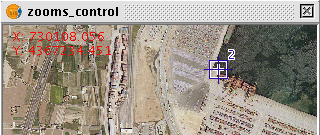
Zoom box associated with the views
Checkpoints
A control point is an entity that provides a correspondence between a geographic coordinate and pixel coordinate. Control points are represented in raster geographic view as Blue-and red circles respectively. To add a new control point is selecting "New" in the table control. This makes a new entry in the table appears. A control point is associated with a table entry. By selecting "New" automatically creates a point at coordinates 0, 0 for both views and will activate the tool "move point". Now clicking on the view point where we will move puncture. We assign the coordinate point numerically by writing directly on the input value in the table (X for the geographic coordinates X, Y geographic coordinate for Y, X 'for X and Y pixel coordinate' for the pixel Y coordinate). The points can also be moved by clicking and dragging on them. This may be done both in hearings and in the zooms.
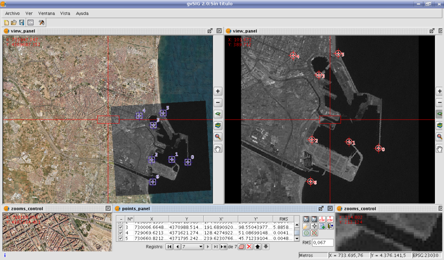
The process of georeferencing. Sights and points of control
Options
The panel labeled "Output File" we must put the path and file name destination if the georeferencing is done with resampling.
The panel georeferencing algorithm "select how we will get the output result. There are two possibilities, "affine transformation" and "polynomial transformation".
The affine transformation applied to raster an affine transformation only to the calculations performed with the control points taken. The affine transformation applied will be allocated on the fly for the display and the output image is the same as the input. The result of this transformation is therefore a georeferencing file. Keep in mind that this type of transformation is limited and the user will be responsible for selecting the most convenient transformation in each case.
The polynomial transformation involves a resampling of the input image taking into account the reference control points and obtaining an output image with deformations necessary to adapt to the new location. If you select this option we will be forced to decide the degree of transformation that we apply and the type of interpolation that we want to apply for calculating new pixels. Depending on whether you choose one degree or another need a minimum number of control points for them. This number of points required is given by the formula (order + 1) * (order + 2) / 2, ie for a polynomial of degree one will be needed at least three points, to grade two will need six points for third grade ten points ... The interpolation method affects the way we calculate the information that we have not. When an image georeferenced output image has deformations with respect to the original there are areas where no information is available. These can not be empty with what must be calculated from the areas where we know. These calculations can be performed by various methods, the simplest of these is "Nearest neighbor" which will be unknown pixel information closest known pixel. Other methods such as "bilinear" or "bicubic" make calculations using the known group of pixels surrounding the unknown. These other methods give a more relaxed but it is slower in its implementation.
The panel "Pixel Pitch" is the pixel size information of the output image. In principle this will be calculated from the input image but can be changed manually.
The panel labeled "Options" contains settings of a different nature. Since we can change the background color of view, the text color of the views. The "show the number of graphically checkpoint" will be displayed or hidden by the control point a point that indicates the corresponding point number. "Add the CSV file errors" will be generated when this type of text files with all the control points we can ignore the file or add the calculated errors. The "Focus the selected point view" makes automatically every time we select a point on the table the view is focused on this. The effect is much as if the tool center point was always active. The "error threshold for the warning," assigns the value at which the error appears in red on the table.
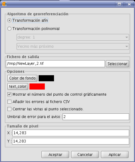
Options for georeferencing
Points Table
The points table is below the sights and initially will be empty. Each table entry corresponds to a checkpoint. It appears all the information related to a point. This table can see it folded its default state or maximized. In its maximized state are folded more information. On the left side of the row there is a check to activate and deactivate the current row. This means that this point will not be displayed graphically or be taken into account for calculation errors and will be prosecuted to do a test. The information can be found in the points table on each point:
- Number of point
- Real coordinate X
- Real coordinate y
- Coordinate pixel X
- Coordinate pixel Y
- Error in X
- Error in Y
- Total RMS error for that point
The quality of the geometric correction can be estimated based on the mean square error RMS error and the contribution of each point. When the contribution to RMS of a point is high, this may indicate that the correspondence of points was poorly selected and the point is not well suited to model transformation between image and map or other information used as reference. The points with high contribution that exceeds a certain threshold can be deleted or deactivated, and calculate the RMS. However, when we are fully confident of the location of a point, and to find you, the RMS is triggered, it may be possible that the geometric model does not resolve the local arrangements, for which they may need a better model, which means, put some more points, right on the problem area.
There is also a global RMS error in an external text field for all points.
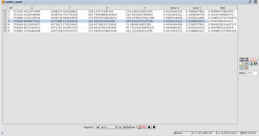
Control Panel points
Controls
Tool center point: When you press the focus control to the view point that is selected.

Georeferencing operation completes. Before you ask if we carry on the gvSIG view the results of the last trial. You'll also want confirmation of application output.

Launching the options dialog.

Make a test with the control points currently entered. If there are not enough for the specified algorithm will warn. The result is that applying the transformation and loading the transformed image on the view with the reference maps.

Save the control points in the metadata file attachment with the raster.

Retrieves the control points that are in the metadata file attached to raster.

Ends the test of processing the raster. Eliminate the test image loaded in the view with the mapping.

When the button "Select point" we are active, clicking on the view assigning the selected point on the table at that time to the position.

Sequence capture control points
There may be ways to capture control points with the tools available. An example would be the following sequence of actions:
- Click "New" in the table of control points. This will create a new row is selected in the table. In addition the tool "Move Point" is selected.
- Click with your mouse pointer over the view to locate the point raster.
- Click with your mouse pointer over the view with reference maps to locate the point.
- Push the button "Refocused selected view point" to place the checkpoint in the center and appears in the zoom window.
- With the tool of choice for area Zoom "or" increase the level of zoom "or" Decrease the zoom level "we can set the desired zoom level until the controls of" Zoom "we have an optimal resolution level approximate.
- Click and drag the control point in the zoom window to place it more precisely. The accuracy depend on how correct is selected previous zoom level.
- Use the zoom tools to return the view to a wider zoom level and to allow a new control point.
- To return to one point and reset the Selection Click on the row of the table, click "Center views the selected point, adjust the zoom level to zoom tools and we'll move the view by clicking and dragging on the window zoom for greater accuracy.
Georeferencing with resampling
Two types of processing for raster. If selected in the options the affine transformation the image obtained is not wide and applies an affine transformation on the view. This transformation is a scaling, displacement, rotation and deformation in the direction of axis X and / or Y axis The transformation with resampling involves generating a new image from the original on which areas can appear empty. These areas are due to the fact that the resulting image should be rectangular but the area covered by the data processing may not have applied this same way.
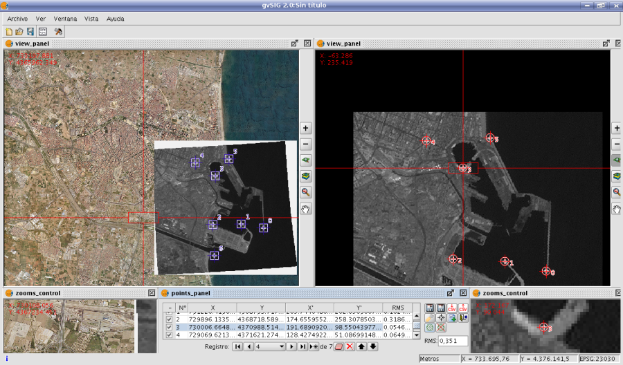
Results georeferenced image with resampling
Once the process of georeferencing the raster generated and loaded in the view we can apply a transparency per pixel to eliminate the empty areas.
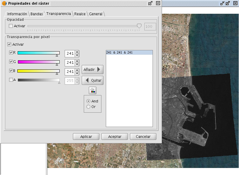
Image georeferenced, with application of transparency
Georeferencing without "Mapping Reference"
The georeferencing without reference maps is useful when you do not have imagery that guide us to assign the control points. We will have to allocate the actual coordinates directly by typing its value. In this case it is useful in view of the left so it will allow more space for the raster and the points table. The operation is very similar to the two views just that when you select the point on the reference maps have to type the entry of the table directly.
The operation of other controls is the same as with reference maps.
