Rossmo’s algorithm
| Package file: | gvSIG-desktop-2.3.1-RossmosFormula-1.0.0-3-testing-all-all-j1_7.gvspkg |
| Code name: | RossmosFormula |
| Version: | 1.0.0-3 |
| Version of gvSIG: | 2.3.1 |
| Type: | Community |
| Owner: | GITS - UNAM, Alexis Jazmín Palomares |
| State: | testing |
| Home page: | |
| Operating system: | all |
| Categories: | Geoprocess |
| Sources: | Browse |
| Description: | |
This tool helps in obtaining a criminal geographic profile through the implementation of the criminological model of Kim Rossmo. |
|
Description
This script generates a points layer which contains the next fields:
ID: a unique identifier for each point.
X: the x coordinate for each point.
Y: the y coordinate for each point.
P: the resultant probability for each point.

The probabilities for the field “P” are computed through the implementation of Rossmo’s algorithm for Geographic Profiling, called, Criminal Geographic Targeting (Rossmo, 2000).
Rossmo’s algorithm can bee seen through the next formula:
where:RossmosFormula/RossmosFormula/
and:
The output is similar to the next image.

Parameters
The parameters required for this tool to work are shown in the next image:

The mandatory parameters are:
Crimes layer: sinces Rossmo’s algorithm is thought to be applied in cases of serial crimes, this points layer will contain the locations related to the specific analyzed case.
Radius of the buffer zone: parameter B in Rossmo’s formula.
k: Value of the constant k in Rossmo’s formula.
f: Value of the exponent f in Rossmo’s formula.
g: Value of the exponent g in Rossmo’s formula.
The optional parameters are:
Probabilities layer: name and location for the output points layer.
Hunting area layer: vector layer of which extreme coordinates (upper right and lower left) are used in order to obtain the extent of the probabilities layer. If no layer is chosen, the extent will be computed according to Rossmo’s algorithm.
Distance between points: this parameter indicates the value of the separation between adjacent points in the probabilities layer. If 0.0 value is used, then this distance will be computed to obtain around 40,000 points in the resultant layer.
Considerations
Some of the factors we need to take into consideration before the execution of this tool are that:
Manhattan distances are computed in order to obtain the probability for every point in the resultant grid, because of this, it is recommended that: crimes layer, hunting area layer (if one were chosen) and the view where these layers are loaded have such coordinate reference system that allows to measure distances. Examples of these reference systems are: UTM or conical projections. As a consequence, users may need to use a projection different from the default one (EPSG: 4326).
The value for the constant k will be used just as a computational aid. This means that if the probablities turns out to be so small, user may assign a big number to this constant, for example: 100 or 1000. In contrast, if lower values are needed, users may assign a small number to this constant.
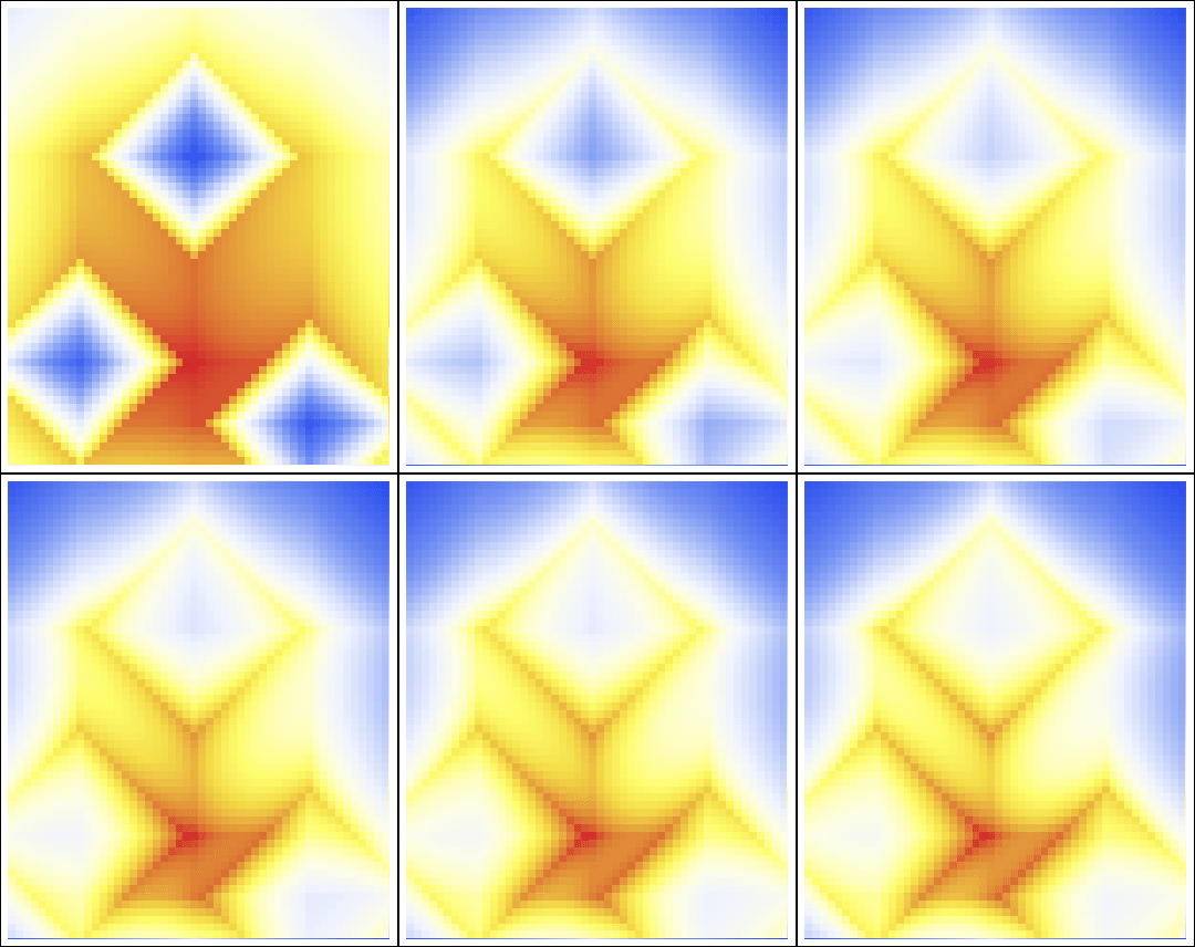
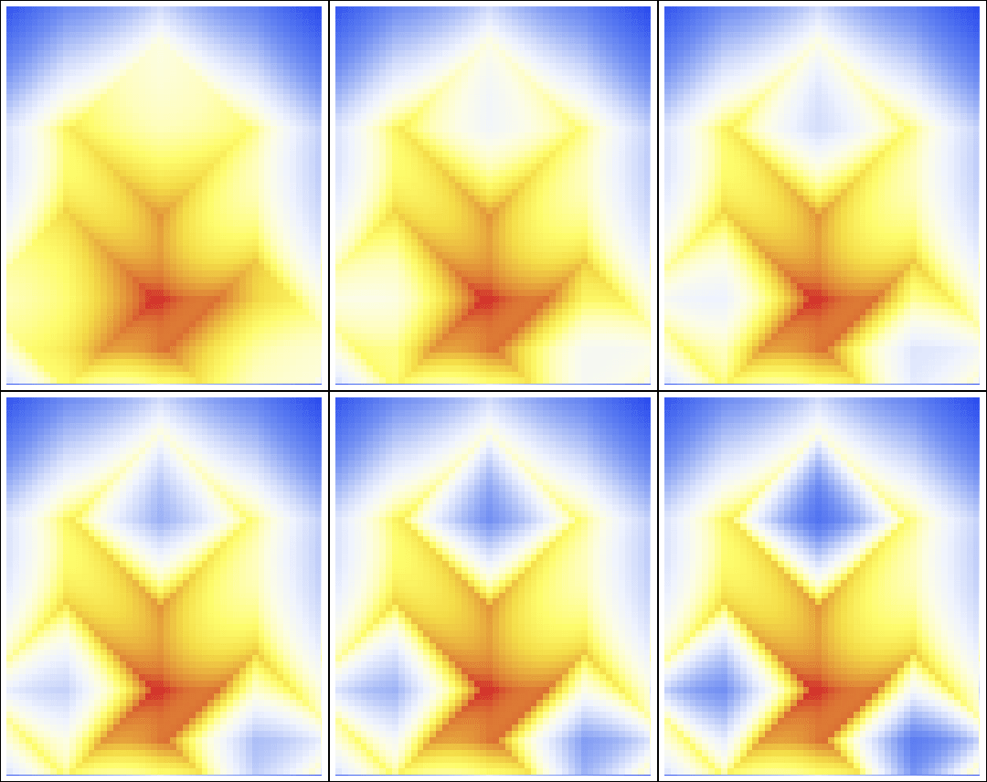
Since the exponents “f” and “g” are used in a distance decay function in order to compute the probability for every resultant point it is important to consider that the greater “f” is, the faster the probability will decay beyond the radius of the buffer zone. This is the main effect of exponent “f”, although its value also affects the probability value inside the buffer zone. On the other hand, exponent “g”, will only affect the values inside buffer zone, it means that the greater “g” is, the faster the probability will decay beyond criminal’s anchor point but exclusively inside the radius of buffer zone.
For further reference on this issue see O’Leary (2011).

Example of the effect in the geoprofile due to a variation of the “f” parameter. In this case “f” goes from 0.1 to 1.25 in steps of 0.05. “g” is fixed at 2/3. (Kun, 2011)

Example of the effect in the geoprofile due to a variation of the “g” parameter. In this case “g” goes from 0.1 to 1.25 in steps of 0.05. “f” is fixed at 2/3. (Kun, 2011)
References
Rossmo, D. Kim (2000). Geographic Profiling. Boca Raton, FL: CRC Press.
Kun, Jeremy (2011). Hunting Serial Killers. Available on: https://jeremykun.com/2011/07/20/serial-killers/ [2017/08/18]
O’Leary, M. (2011). Modeling criminal distance decay. Cityscape, 161-198.
